Team:EPFL/Model

iGEM EPFL 2016

Model

In order to be able to predict the output and reliability of each biological circuit, Cello requires that each gate have a defined response function, that predicts the output of that gate’s output promoter based on the strength of the input promoters. Since many of our gates are modifiable and would not rely on the simple “tandem promoter” architecture that Cello uses, gate response functions would have to be predicted based on the response functions of individual parts, when they are not known. Since each part has the same general structure, it is possible to develop a general model for each part, from which a response function for the gates output can be extracted.

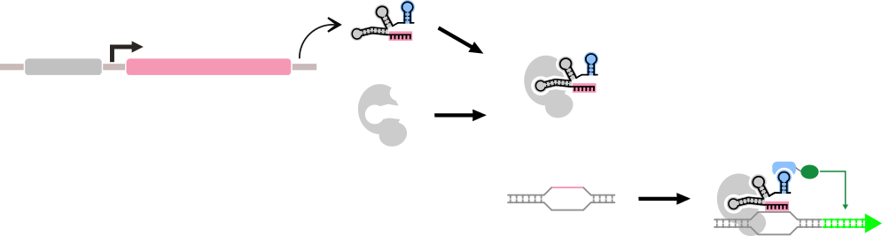
Part representation — The general form of a dCas9-based "Part" that we are considering here. A part in this context is composed of multiple genetic components, but has a single repsonse function.

Originally, we hypothesized that these factors were important for determining the response function of a part:

The strength or response function of the input promoter.
The selective binding of dCas9 to the target sequence.
The interaction between the specific output promoter and the specific transcriptional effector for that target.

Additionally, we made the following hypotheses:

The binding of the guide RNA(gRNA) to the dCas9 is equally efficient for all guide sequences, and the change in target sequence does not affect the binding of the promoter effector module (PEM). This protein effector module is composed of an RNA-interacting domain, which binds to the scRNA, and a transcriptional effector domain. Here, gRNA is used to describe both single guide RNAs (sgRNA) and scaffold RNAs (scRNA). This model does not consider guides which have to be assembled from crRNA and tracrRNA. In this case, an extra step describing the rate of assembly would have to be included.
The binding constant of dCas9-gRNA-PEM with its target DNA is much greater than the dissociation constant.
Targets with a Gibb’s free energy of binding (ΔG_target) of -4 kCal/mol or more would take 6 days or more to bind within the system and so could be ignored. The normal binding energy for a target is under -9 kCal/mol (Farasat & Salis, 2016).

In this case this system can be described as a system of ordinary differential equations:

We must first model the formation of the dCas9-sgRNA-PEM complex. We assume that the formation of this complex reaches a rapid equilibrium. Therefore the amount of bound dCas9-guide RNA c omplex that exists can be described as a function of the on-rate of this complex, multiplied by the concentrations of the subparts of the complex, and the off-rate of the complex, multiplied by its concentration:

$$C_B=k_1*gRNA*C_F *PEM-k_2C_B$$

A graphical representation of the kinetics of the assembly of the sgRNA-dCas9-PEM complex.
1. $C_B$: The concentration of bound dCas9-gRNA-PEM complex.
2. $gRNA$: The concentration of gRNA for the given target.
3. $C_F$: The concentration of free dCas9
4. $PEM$: The concentration of Protein Effector Module. This module contains an RNA binding module, and a transcriptional effector module. The RNA binding module binds to the added hairpin of the scRNA.
5. $k_1$: The on-rate for the dCas9-gRNA-PEM complex.
6. $k_2$: The off-rate for the dCas9-gRNA-PEM complex.
This equation is tied to the following equations. The amount of free dCas9 can be described in terms of the rate of formation of the dCas9 (which we consider to be constant while the circuit is running), the sum of the rates of formation of dCas9-gRNA-PEM complexes for all the targets used in the system, and the rate of degradation of the dCas9. We can also describe the concentration of the gRNA for a particular target in terms of the activity of its promoter (which will have a certain response function) and the rate of degradation of the gRNAs, multiplied by the concentration of the gRNA.

$$C_F=r_{dCas9}-\sum_i k_1gRNA_iC_FPEM+k_2C_B-k_3C_F$$ $$gRNA= r_gRNA (x)-k_4 gRNA$$
1. $r_{dCas9}$:The rate of dCas9 production in this system, when the circuit is running. This could be determined by a constitutive promoter, or by the output promoter of a switch if the circuit has a master switch.
2. $\sum_i k_1gRNA_iC_FPEM$: The sum of all of the rates of formation for all possible dCas9-gRNA-PEM complexes. This term accounts for the reduction in binding rates that occurs when free dCas9 is sequestered by particular gRNAs to the detriment of the formation of other complexes.
3. $k_3$: The degradation rate of the free Cas9.
4. $r_gRNA (x)$: The rate of transcription of the particular gRNA, which is dependent on the strength of the promoter and the “input” to the promoter, or the concentration of transcriptional effectors, their effects, and their strengths. These inputs are modeled as$x$.
5. $k_4$: The degradation rate of the gRNAs. We suppose that all gRNAs have the same degradation rate.
Once the binding of the dCas9-gRNA-PEM complex is modeled, we can approach the binding of this complex to its target DNA. In addition, it may be interesting to note here that the binding of dCas9 to its target DNA occurs more often than Cas9 to the same target, and that the binding of dCas9 to a promoter is proportional to the basal activity of that promoter (Farasat & Sallis, 2016). The on-rate can be affected by the presence of other dCas9-gRNA-PEM complexes bound near the target site, although there is steric hindrance immediately next to the target site when dCas9 is bound, there is also a supercoiling effect, since the dCas9 unwinds the DNA at its target site, increasing the tension in the DNA nearby, making it more difficult for other dCas9s to similarly open the DNA. Close to the target site this effect is additive and linear in terms of the change in binding energy, but becomes unimportant at a distance of about 200bp from the target site (Farasat & Sallis, 2016). Before we can model the proportion of the bound promoter we must consider how the on- and off- rates of the DNA-dCas9-gRNA-PEM complex will be affected by this supercoiling.

We know that the supercoiling changes the binding energy according to the formula (Farasat & Sallis, 2016): $$ΔG_{supercoiling} = -10lnk_b T(σ_F^2 - σ_I^2)$$
1. $σ_F$: The superhelical density of the DNA around the target sequence after dCas9-gRNA-PEM binding.
2. $σ_I$: The superhelical density of the DNA around the target sequence before dCas9-gRNA-PEM binding.
3. $n$: The number of base-pairs that were unwound.
4. $k_b$: The Boltzmann constant.
5. $T$: The temperature in Kelvin
6. $l$: The number of bound target sites in the neighborhood of the particular target being considered.
Because of the exponential relationships that exists between binding energy and on- and off- rates, the relationship between the on-rate of the DNA-dCas9-gRNA-PEM complex can be described as a function of the on-rate in the absence of supercoiling, and the change in energy in the presence of supercoiling.
The factor by which the on- and off- rates change can be described by the following equation: $$e^\frac{-ΔG_{supercoiling}}{k_b T}$$
We also know that the average amount of supercoiling in the yeast genome is -0.05 (Roca, 2011), and that n=23. We therefore have the following relationship between the on-rate of the DNA-dCas9-gRNA-PEM-PEM complex when we account for supercoiling and the original: $$k_{5,supercoiling} = \sum_{l=0}^j \frac{l!}{(j-l+1)!l!}*\frac{k_5 *p}{e^{230l(σ_F^2 -0.0025)}}$$ Similarly: $$k_{6,supercoiling} = \sum_{l=0}^j \frac{l!}{(j-l+1)!l!}*\frac{k_6 *e^{230l(σ_F^2 -0.0025)}}{p}$$
1. $k_5$: The maximum on-rate for a DNA-dCas9-gRNA-PEM complex in the system.
2. $k_{5,supercoiling}$: The on-rate of the DNA-dCas9-gRNA-PEM complex when we account for supercoiling.
3. $k_6$: The maximum off-rate for a DNA-dCas9-gRNA-PEM complex in the system.
4. $k_{6,supercoiling}$: The off-rate of the DNA-dCas9-gRNA-PEM complex when we account for supercoiling.
5. $l$: The number of supplementary binding sites for dCas9 in the neighborhood of the target that are bound.
6. $j$: The total number of supplementary binding sites for dCas9 in the neighborhood of the target.
7. $p$: The relative activity of the promoter in the target. $p \in{]0,1]}$ where $p=1$ for the most active promoter in the system.
Now we can model the amount of bound promoter in a system in terms of the on- and off- rates that account for supercoiling and the concentration of the dCas9-gRNA-PEM complex: $$P_B=k_{5,supercoiling}C_B P_F-k_{6,supercoiling}P_B$$ $$P_B+P_F=1$$

A graphical representation of the binding of the dCas9-gRNA-PEM complex to the target sequence.
1. $P_B$: The proportion of bound target promoter.
2. $P_F$: The proportion of free target promoter.
Practically, since we know that the affinity of binding is very high between dCas9-gRNA-PEM and the target DNA, even very low concentrations of dCas9-gRNA-PEM will suffice to drive $P_B \rightarrow 1$. When supercoiling in the DNA exceeds a certain point, the tension in the DNA double helix will drive the off-rates of the targets to approach the on-rates and certain targets will remain on-average, unbound, depending on their positions relative to the others. It is important to note that this model depends on the specificity of binding of the dCas9, and that there is very little off-target activity. To ensure that this would be the case in our system, we designed a serious of guides using the Platform DESKGEN. Head here to find out more about what we did!
In the final part of the model for the parts, we describe the amount of product which is present in the system. We describe this concentration in terms of the rate of break-down of the product, the effect of the effector on the promoter, and the proportion of the target promoter that is bound:

If the effector is a repressor: $G=αP_F+β-κ_7 G$

If the effector is an activator: $G=γP_B+δ-κ_7 G$
1. $G$: The concentration of the product.
2. $α+β$: The production rate of the product when the target promoter is completely unbound, in the case of a transcriptional repressor.
3. $β$: The production rate of the product when the target promoter is completely bound, in the case of a transcriptional repressor.
4. $γ+δ$: The production rate of the product when the target promoter is completely bound, in the case of a transcriptional activator.
5. $δ$: The production rate of the product when the target promoter is completely unbound, in the case of a transcriptional activator.
6. $k_7$: The degradation rate of the product.
Let us now consider the role of parts that link to other parts. Most parts have input values below which they are definitively “off” and above which they are definitively “on”. These inputs can come in the form of gRNAs. In order to simplify our model, while keeping it realistic, we will imagine that no product $G$ is produced when the output would be below this lower threshold (and therefore the next part would be “off”), that it is produced when the input is above the upper threshold (and therefore the next part would be “on”), and we will not treat the “undefined” case in-between.

Therefore, if the effector is a repressor: $$G = \begin{cases} \text{consider G=0 in next steps}, & G \leq t_{off} \\ αP_F+β-κ_7 G, & G \geq t_{on} \\ \end{cases} $$ and if the effector is an activator: $$G = \begin{cases} \text{consider G=0 in next steps}, & G \leq t_{off} \\ γP_B+δ-κ_7 G, & G \geq t_{on} \\ \end{cases} $$
1. $t_{on}$: The lowest input value for $x$ when the production rate of gRNA is high enough for the promoter to be predictably on.
2. $t_{off}$: The highest input value for $x$ when the production rate of gRNA is low enough for the promoter to be predictably off.

From Part to Gate

A gate can be thought of as a sequence of parts. Therefore, the response function of a gate can extrapolated from the response functions of the component parts by determining whether the output of one part is sufficiently high to “trigger” the next part. If it is, the next part is considered to be “on”, and so on and so forth. If the output of the gate is not sufficiently high, the next part will be in an “off” state.

As most gates combine multiple inputs, there are certain parts which will have multiple inputs. In the case of parts where the multiple inputs have the same function, the effects can be additive and the threshold higher. For example for a system where two products $G$ and $H$ would go on to form a complex that would activate another promoter, if the concentrations of $G$ and $H$ would be additively too low to turn the promoter on, then we would consider their effective concentrations to be null. They could even act differently on the promoter, which could be modeled by giving them two different parameters: and , for example. Written mathematically:

If the effectors are repressors: $$ G,H = \begin{cases} \text{consider G,H = 0 in next steps}, & q_G G+q_H H \leq t_{off} \\ α_G P_{F,G}+β_G-κ_7 G,α_H P_{F,H}+β_H-κ_7 H, & q_G G+q_H H\geq t_on \\ \end{cases} $$ In the case when transcriptional activators and repressors act on the same promoter, we consider that the repressor beats the activator, so we consider only the effect of the repressor. This has been reported in the literature (Gilbert et al., 2014) and we also confirmed it experimentally in our project.

implementation

The implementation of this model is fairly straightforward. The first step of this model involves the identification of the parameters. After identifying the $t_{on}$ and $t_{off}$ rates of the circuit output promoters, these values can be mapped onto the promoters one step earlier in the circuit to give $ t_{off}^{'} $ and $ t_{on}^{'} $. These values represent the activation of the promoters directly before the aforementioned output promoters necessary to ensure the “on” and “off” states of these promoters. This method is repeated throughout the circuit until these values are identified for the input promoters to the circuit. At this point input values lower than these lower threshold values identified for the input promoters will represent 0 – or negative - inputs, and input values higher than the upper threshold values will represent 1 – or positive inputs. We have not yet had an opportunity to integrate this model into our database to generate response functions for our gates, but (time permitting), we will do this after wikifreeze!

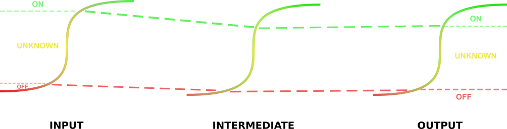
"Tracing" the $t_{on}$ and $t_{off}$ values back through the parts.

References

Gilbert, Luke A. et al. “Genome-Scale CRISPR-Mediated Control of Gene Repression and Activation.” Cell 159.3 (2014): 647–661. PMC. Web. 17 Oct. 2016.
Roca, Joaquim. “Transcriptional Inhibition by DNA Torsional Stress.” Transcription 2.2 (2011): 82–85. PMC. Web. 17 Oct. 2016.
Farasat, Iman, and Howard M Salis. “A Biophysical Model of CRISPR/Cas9 Activity for Rational Design of Genome Editing and Gene Regulation.” PLOS Computational Biology, 19 Jan. 2016, http://dx.doi.org/10.1371/journal.pcbi.1004724.