Team:HZAU-China/Model

Model
1. Circuit Dynamic Model
1.1 Bacteria motility and CheZ protein
The phosphorylation of CheY causes the bacteria to tumble, and CheZ can promote CheY's dephosphorylation, which makes the bacteria move forward.
1.2 Chemotaxis model
In the experiment, we use the green light to irradiate the bacteria, control the phosphorylation of CcaS, and lead to the phosphorylation of CcaR. The phosphorylation of CcaR can promote the expression of PleD, which plays a key role in the enzymatic synthesis of c-di-GMP.
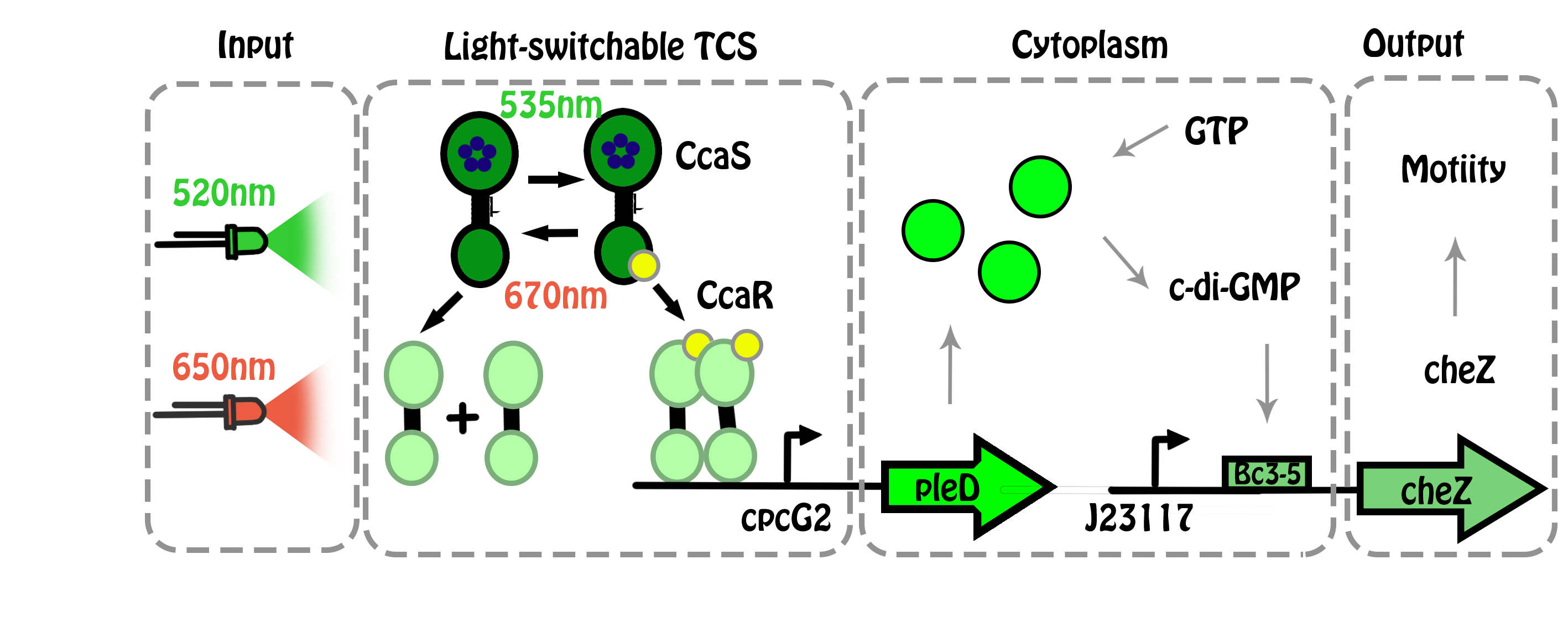
Figure 1. Gene circuit.
The concentration of c-di-GMP has a very close relationship with the triple-tandem riboswitches efficiency, the specific relationship is as following:
\(R(single)=\frac{C_{(c-di-GMP)}}{T_D + C_{(c-di-GMP)}}\), (1)
\(R(double)=[\frac{C_{(c-di-GMP)}}{T_D + C_{(c-di-GMP)}}]^2\), (2)
\(R(triple)=[\frac{C_{(c-di-GMP)}}{T_D + C_{(c-di-GMP)}}]^3\). (3)
In equation (1), (2), (3), \(T_D\), the equilibrium constant, equals to the c-di-GMP concentration \(C_{(c-di-GMP)} \) at 50% read-through rate [2].
Due to efficiency of the triple-tandem riboswitches, we can finally know the expression level of cheZ, so the relationship between PleD and CheZ concentration can be investigated. The model is based on the assumption that the expression of PleD is certain and can immediately respond to certain light. Because in E.coli, GTP, the substrate of PleD, is sufficient, so that the enzymatic reaction rate for producing c-di-GMP is regarded as at the stable rate \(\kappa\). \(\alpha\), \(\alpha_2\) represent for the degradation rate of PleD and c-di-GMP respectively. \(\beta_1\) represents for the synthetic rate of PleD, \(C_{0(CheZ)}\) represents the initial concentration of CheZ. (Equation 4 )
$$ f(x)=\left\{ \begin{aligned} \frac{C_{(PleD)}}{dt} & = & \beta_1 - \alpha_1 \times C_{(PleD)} \\ \frac{C_{(c-di-GMP)}}{dt} & = & \kappa - \alpha_2 \times C_{(c-di-GMP)}, &\ \ \ \ \ \ \ \ (4) \\ C_{(CheZ)} & = & R \times C_{0(CheZ)} \\ \end{aligned} \right. $$
1.3 Conclusion
The stimulation result is as the following:
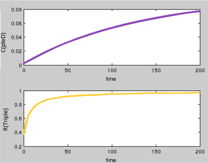
Figure 2. Green light.
The efficiency of the triple-tandem riboswitches and the concentration of PleD both have a significant positive correlation with the concentration of c-di-GMP. The concentration of pleD keeps on increasing, and finally the efficiency of the triple-tandem riboswitches can reach up to 100% (Figure 2).
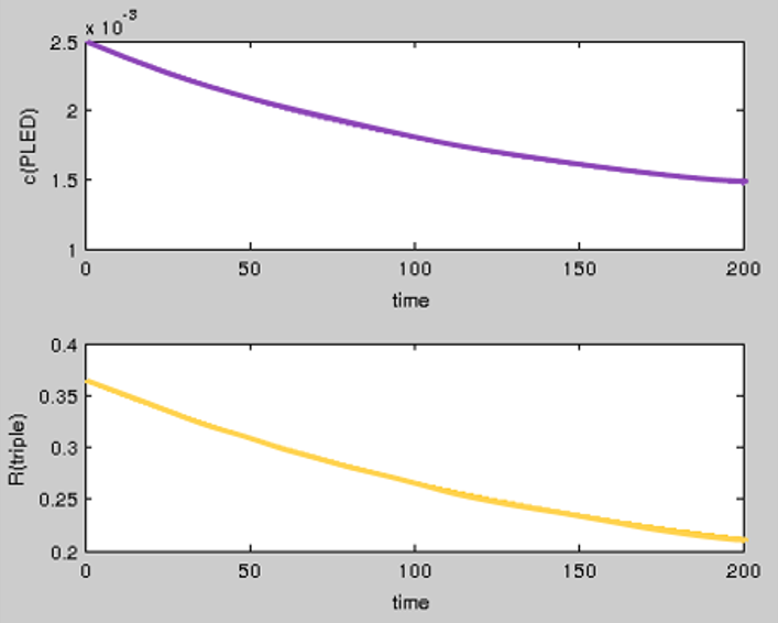
Figure 3. Red light.
When simulation of colony is under the irradiation of red light, the concentration of PleD decreased slowly. Because of that, the responding time of riboswitches is short. With the incessant decrease of PleD, the open efficiency of riboswitches will reduce to a stable value (Figure 3).
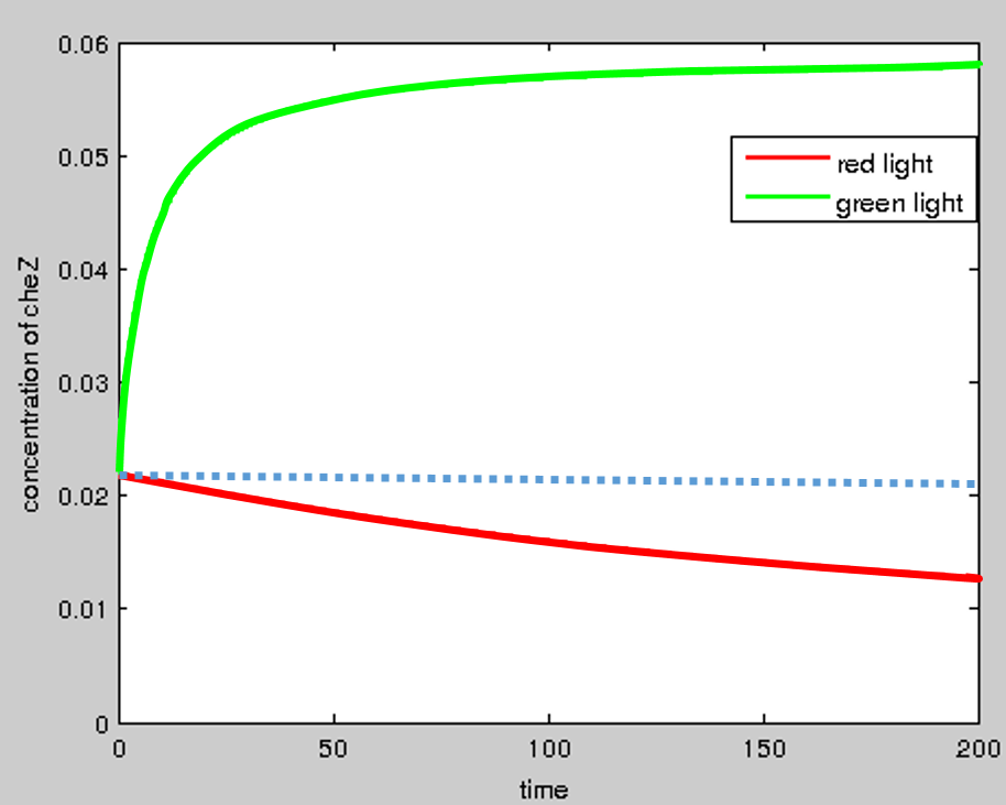
Figure 4. The concentration of CheZ.
The concentration of CheZ is significantly affected by the riboswitches. The model shows that under the irradiation of red light and green light, the concentration of CheZ has a significant difference, enough to control the motility of bacteria to form certain bio-pattern (Figure 4).
2. Reproduction-Motion Model
The distribution density of bacteria in a culture medium depends on two factors: motion and reproduction of bacteria. For convenience, we will discuss these two factors separately.
2.1 Dynamic model of bacteria motion
In this project, we are trying to control the motion of bacteria by light signal to generate a colony of a specific shape. The light signal can affect the bacteria motility by influencing the expression of a protein cheZ. There are two motion forms of bacteria: tumbling and swimming. By tumbling, bacteria can change swimming direction but not position; by swimming, bacteria will move forward and change the position. In fact, the ratio of tumbling to swimming is different from one bacterium to another. At the microscopic level, the angle of tumbling is random, so we have no idea about the movement direction of a bacterium in any time. But from a macroscopic viewpoint, the probability of all directions are equal. This property is similar to the diffusion of a chemical molecule. So, bacteria swimming can be treated as the diffusion of bacteria and the rate of diffusion is related to the expression of protein cheZ.
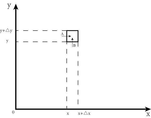
Figure 5. The 2D plane of bacteria diffusion.
In Figure 5, the simple square represents the area of bacteria in coordinate \((x,y)\) approximately. The number of bacteria in this area is \(S(x,y,t)\) at time t. So, we have
\(S(x,y,t)=\rho(x,y,t)*\Delta x\Delta y\). \((5)\)
In Equation \((5)\), \(\rho(x,y,t)\) represents the bacteria density in that area. \(\Delta x\) and \(\Delta y\) are the small increments along the \(x\) and \(y\) axes, respectively. Taking the derivative of Equation (5), we have
\(\frac {\partial S(x,y,t)}{\partial t}=\frac {\partial\rho(x,y,t)*\Delta x\Delta y}{\partial t}\). \((6)\)
The left side of Equation \((6)\) represents the change rate of \(S(x,y,t)\). Ignoring the reproduction of bacteria, the change rate depends only on the rate of bacteria diffusion. As shown in Figure 5, bacteria can move along the \(x\) axis and the \(y\) axis. Suppose the movements along the \(x\) and \(y\) axes are positive, we arrive at
\(\frac {\partial\rho (x,y,t)\Delta x\Delta y}{\partial t}=\phi_x(x,y,t)\Delta y- \phi_x(x+\Delta x,y,t)\Delta y+\phi_y(x,y,t)\Delta x-\phi_y(x,y+\Delta y,t)\Delta x\). \((7)\)
In Equation \((7)\), \(\phi_x\) and \(\phi_y\) represent the diffusion of bacteria in \(x\) and \(y\) axes, respectively. Dividing \(\Delta x*\Delta y\) on both sides of Equation \((7)\), and we can get
\(\frac {\partial\rho(x,y,t)}{\partial t}=\frac {\phi_x(x,y,t)-\phi_x(x+\Delta x,y,t)}{\Delta x}+\frac {\phi_y(x,y,t)-\phi_y(x,y+\Delta y,t)}{\Delta y}\). \((8)\)
Let \(\Delta x\) and \(\Delta y\) take a limit to 0, Equation \((8)\) will become
\(\frac {\partial\rho(x,y,t)}{\partial t}=\lim_{\Delta x\rightarrow 0}\frac {\phi_x(x,y,t)-\phi_x(x+\Delta x,y,t)}{\Delta x}+\lim_{\Delta x\rightarrow 0}\frac {\phi_y(x,y,t)-\phi_y(x,y+\Delta y,t)}{\Delta y}\). \((9)\)
This equation is equivalent to
\(\frac{\partial \rho}{\partial t}=-(\frac{\partial\phi_x}{\partial x}+\frac{\partial\phi_y}{\partial y})\). \((10)\)
In this equation, \(\phi_x\) and \(\phi_y\) are unknown. In fact, the diffusion rates along \(x\) and \(y\) axes are the same. Refer to the assumption of Fourier Heat Equation:
1. If the temperature is constant within an area, there is no flow of heat.
2. If temperature difference exists in adjacent areas, heat will flow from areas of high temperature to low temperature.
3. For the same kind of material, the bigger the temperature difference between two adjacent areas, the faster the heat flow between them.
We have three similar characters for the diffusion of bacteria colony:
1. If the density of bacteria is constant in an area, the movement of bacteria will not lead to the change of density.
2. If density difference exists in adjacent areas, bacteria will swim from high density to low density areas.
3. The bigger the density difference between two adjacent areas, the faster the diffusion rate between them.
So, the rate of diffusion is related with the difference of density:
\(\phi_x = -k\frac{\partial\rho}{\partial x}\), \((11)\)
\(\phi_y = -k\frac{\partial\rho}{\partial y}\). \((12)\)
Combining Equation\((10)\), Equation\((11)\) and Equation\((12)\), we can get
\(\frac{\partial\rho}{\partial t} = k(\frac{\partial^2\rho}{\partial x^2}+\frac{\partial^2\rho}{\partial y^2})\). \((13)\)
Equation (13) is the dynamic model of bacteria motion.
2.2 Dynamic model of bacteria reproduction
There is a famous model about the growth of bacteria under the conditions of limited space and nutrients, called logistic growth model:
\(\frac{d\rho}{dt} = \gamma\rho(1-\frac{\rho}{\rho_s})\). \((14)\)
In Equation \((14)\), \(\rho\) represents the density of bacteria, and \(\gamma\) is the growth rate constant, and \(\rho_s\) is the saturated density.
2.3 Dynamic model of both reproduction and motion (R-M model)
Combining equation \((13)\) and equation \((14)\), we have
\(\frac{\partial\rho}{\partial t}=k(\frac{\partial^2\rho}{\partial x^2}+\frac{\partial^2\rho}{\partial y^2})+\gamma\rho(1-\frac{\rho}{\rho_s})\). \((15)\)
Referring to the paper by Liu et al. [1], we have the parameter values:
$$k=200~1000\mu m^2/s,$$ $$\gamma = 3.89e-4s^{-1},$$ $$\rho_s = 1500cell/\mu m^2.$$
We will use the Finite Element Method to solve this PDE. Initial conditions are defined as
$$\rho=matrix.zeros(200,200),$$ $$\rho[100,100]=100,$$
where \(matrix.zeros(200, 200)\) means a zero matrix with \(200*200\) elements and the initial value of the element at the index \([100, 100]\) of this matrix is \(100\). And the boundary conditions are
$$\rho[0:,]=0,$$ $$\rho[100:,0]=0,$$ $$\rho[0,0:]=0,$$ $$\rho[0,100:]=0.$$
With the initial and boundary conditions, Equation \((15)\) was solved by writing python program with Numpy and the result was visualized by the Mayavi python package, as shown in the following video (Movie 1).
Movie 1. Visualization for the R-M model of bacteria diffusion.
2.4 R-M model in a restricted area
In Movie 1, we can see that bacteria colony will eventually become a round shape. If we add a restrictive condition to the area to limit the bacteria movement, what shape will the bacteria colony become? The way to add area limit in our project is using light signal to control the motility of bacteria. Namely, green light is given to a specific area and red light is given to other area; bacteria can only move in the green light area. In Equation (15), bacterial motility is reflected by parameter k. So the model will be the following equations:
\(\frac{\partial\rho}{\partial t}=k(\frac{\partial^2\rho}{\partial x^2}+\frac{\partial^2\rho}{\partial y^2})+\gamma\rho(1-\frac{\rho}{\rho_s})\), \((11)\)
\(k=f(x,y)\). \((16)\)
The parameter \(k\) in Equation \((15)\) indicates the diffusion rate of the bacteria colony. \(f(x,y)\) is the area limit function, and it is an image matrix. In this project, we choose Pikachu (a famous cartoon character in the hot AR game "Pokimon Go") as our target pattern. See Figure 6.

Figure 6. Pikachu,a famous cartoon character.
The black part in Figure 6 means that the parameter \(k\) is of normal value. That is, \(k=k_{normal}=200~1000\mu m^2/s\). The white part in Figure 6 means that the parameter \(k\) takes small value which will be set to \(0\). Because \(k\) is a matrix in Equation \((11)\), it can be solved out by using Figure 6:
$$k = img*k_{normal}/255.$$
Under the aforementioned initial and boundary conditions, using python program to solve these equations, we can get the following visualization video (Movie 2).
Movie 2. Visualization for the R-M model of bacteria diffusion in a restricted area using Pikachu as the target pattern.
From Movie 2 we can see that the target pattern is basically formed. However, such a pattern formation is just equivalent to making a cookie using a mould. In this project, the pattern formation process will be regulated by a computer by real-time communication.
2.5 R-M model with dynamic regulation
Area limit is a kind of static regulation, but dynamic regulation is further explored in our project. In dynamic regulation, we will compare the shape of the bacteria colony with the target picture by real-time communication between the computer simulated virtual space and the real space in the culture medium through light, and the result of comparison will be converted to light signals shedding on the bacteria colony to control bacteria diffusion. So, the dynamic model with regulation will like the following equations:
\(\frac{\partial\rho}{\partial t}=k(\frac{\partial^2\rho}{\partial x^2}+\frac{\partial^2\rho}{\partial y^2})+\gamma\rho(1-\frac{\rho}{\rho_s})\), \((15)\)
\(k=f(t,\rho,img)\). \((17)\)
Unlike Equation \((16)\), there are two additional parameters in Equation \((17)\). The two additional parameters are time \(t\) and density \(\rho\), respectively. That means parameter \(k\) will change in the pattern formation process by adjustment. Equation\((17)\) can be interpreted as:
\(\rho_1=\rho*\frac{255}{max(\rho)}\), \((18)\)
\(\rho_2=threshold(\rho_1,THRES\_BINARY\_INV)\), \((19)\)
\(edges=Canny(\rho_2)\), \((20)\)
\(edges_2=bitwise\_and(edges, mask=img)\), \((21)\)
\(k_1=dilate(edges_2.kernel)\), \((22)\)
\(k_2=bitwise\_and(k_1,mask=img)\), \((23)\)
\(k=k_2*\frac{k_{normal}}{255}\). \((24)\)
Equations \((18)\rightarrow(24)\) are written in OpenCV language. Equation \((18)\) is for transforming the matrix of bacteria colony to an image. Equation \((19)\) is for image binaryzation. Equation \((20)\) is for finding the edge of an image. Equation \((25)\) is for comparing the current image with the target image. Equation \((22)\) is for expanding the edge. Equation \((23)\) is to prevent overflow from the edge. Equation \((24)\) transforms the result of Equation \((23)\) to light signal. Under the aforementioned initial and boundary conditions, using python program to solve these equations, we can get the result.
Movie 3. Visualization for the R-M model of bacteria diffusion with dynamic regulation using Pikachu as the target pattern.
You can download all the modeling programs from here.
3. Cellular Automaton Model
Our project aims at establishing a computer-guided bio-pattern formation system by deceiving the chemical sense of bacteria. We control the light to mislead the bacteria with the help of the computer so as to achieve the goal of automatically control the bacterial movement. In order to form a specific pattern of bacteria, the bacteria’s distribution in the system can be monitored and controlled in real-time by computer. We use personal computer to get the pictures of the colony, and compare the image with the target pattern.
3.1 Cellular automaton model to simulate the pattern formation of colonies
The cellular automaton is a discrete model studied in computability theory, mathematics, physics, complexity science, theoretical biology and microstructure modeling, Cellular automaton model has three main characteristics
1: parallelism: each unit cell is simultaneously synchronized to change. The state of cell at \(t+1\) time depends on the state of the cell itself and its neighboring cells at \(t\) time.
2: consistency: all cells are governed by the same rules.
3: locality: change of cell state only depends on the state of its neighboring cells.
Because the model is a simulation of bacterial reproduction, Moore neighbors is more identical to the reality, and is conducive to the analysis of the problem, so we use Moore type of neighbors for simulation.
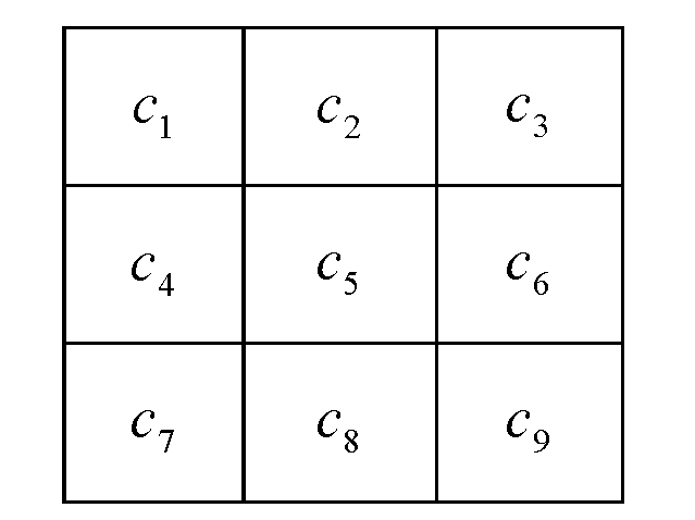
Figure 7. Moore neighbors.
Main steps of image recognition algorithm
1. Image acquisition.
2. Transforming colored images into gray images.
3. Edge detection and extraction (by Canny operator).
4. Comparison between colony image and target image.
5. Regulate the light according to the results.
6. Show the simulation results.
3.2 Mathematical model of bacteria breeding process
In the breeding process, bacteria are mainly affected by two key parameters, the number of bacteria and nutrients. When the nutrient is sufficient, the growth of bacteria can be divided into four stages.,The adaptation period \((0,P_1]\), the growth period \((P_1,P_2]\), the stable period \((P_2,P_3]\), and the death period \((P_3,\infty)\), as shown in Figure 8. During the adaptation period, the bacteria cannot fully adapt to the environment, so the growth is slow; during the growth period, the situation of bacteria is better. So bacteria can rapidly grow exponentially; during the stable period, the reproduction rate and death rate are nearly equal to each other, so the number of the bacteria remains relatively stable; during the death period, due to the accumulation of toxins and many other factors, the amount of bacteria begin to decrease.
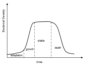
Figure 8. Breeding process.
3.3 Bacteria growth
We assume that the nutrient medium distribution is two-dimensional, the number of bacteria is related with its location parameter \((i,j)\) , as well as time parameter \(t\), then the number of bacteria is defined as \(B(i,j,t)\), in this model i∈{0,1,2…n}i∈{0,1,2…n} \(i\in\{0,1,2 \ldots n\}\) , \(j\in\{0,1,2 \ldots m\}\) , \(t\in\{0,1,2 \ldots \infty\}\) , \(n\) and \(m\) are the length and width of the model.
For a single cell, no bacteria exist at the initial state. When under the control of simulated light, the bacteria will accelerate movement, and the movement of bacteria is not directional, so the edge of the bacteria colony will move to the neighbor cells.
The mathematical model of bacterial growth is as following[3]:
$$ B(i,j,t+1)=\left\{ \begin{array}{rcl} B(i,j,t) \times \alpha + \mu_1 & & {0 < t \leq P_1 }\\ B(i,j,t) \times \beta + \mu_2 & & {P_1 < t \leq P_2\ \ \ \ \ \ \ \ \ \ \ (25)} \\ B(i,j,t) + \mu_3 & & {P_2 < t \leq P_3 }\\ B(i,j,t) \times \frac{1}{\lambda} + \mu_4 & & {P_3 < t < \infty\ \ \ \ .} \end{array} \right. $$When the cellular nutrition is sufficient, the cellular initial distribution is defined at time \(0\). When in the adaptation period, the number of bacteria increases slowly, growth rate equals \(\alpha\). The number of bacteria increases rapidly in the growth period, growth rate equals \(\beta\). Stable period does not change the number of bacteria, while in death period bacteria are fast to reduce,death rate equals \(\lambda\). \(\mu\) is based on the cellular state of the pseudo-random number (Equation 25). Random changes in the scope of the amount of bacteria are in accordance with the period of change.
3.4 Mathematical model of bacteria movement
Since the Moore type of neighbors are used for simulation (Figure 7), the direction of bacterial movement is uncertain. When the edge of bacteria colony is irradiated with light, each bacterium has the same probability to move to other locations. So we have:
\(B(i+h_1,j+h_2,t)=B(i+m,j+n,t)+B(i,j,t) \times \gamma \) \((h_1 \in {(-1,0,1)} \ , \ h_2 \in {(-1, 0, 1)})\) , (26)
\(B(i,j,t)=B(i,j,t) \times (1-\gamma) \) . (27)
In equation (26), \(\gamma\) represents for the probability of the bacteria to swim away, \(B(i,j,t)\) represents for the number of bacteria at the position \((i,j)\) at time \(t\), \(B(i+h_1,j+h_2,t)\) represents for the position the bacteria swim to at time \(t\)
3.5 CA model in a restricted area
During the process of colony recognition, edge extraction of bacteria is processed only within the target area. It is assumed that red light repression on bacterial motility is executed in the other area. So they can only reproduce at the current position, rather than swim or diffuse to other locations.
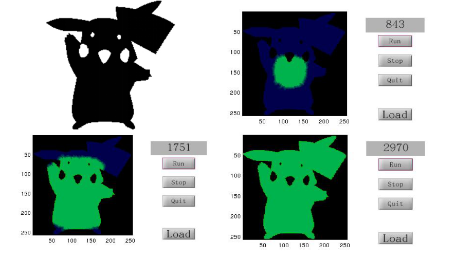
Figure 9. CA program.
In the model, initial inoculation position can be acquired by clicking the desired point in the picture with a mouse and then program can initiate. After a series of simulation, an optimized initial inoculation position can be found, and further help the pattern formation of the bacterial colony.
References
1. Chenli liu, et al. Sequential Establishment of Stripe Patterns in an Expanding Cell Population. Science 334, 238. (2011)
2. Zhou, Hang, et al. "Characterization of a natural triple-tandem c-di-GMP riboswitch and application of the riboswitch-based dual-fluorescence reporter." Scientific reports 6 (2016).
3. Kreft, Jan-Ulrich, Ginger Booth, and Julian WT Wimpenny. BacSim, a simulator for individual-based modelling of bacterial colony growth. Microbiology 144.12 (1998): 3275-3287.