Purdue Biomakers

Modeling

Introduction

Performance of the system was predicted using a finite difference model. To purpose of the model is to inform design regarding the viability of the PAO system, particularly to predict how long a single PAO reactor is useful before needing to induce the phosphate export subsystem.

Methods

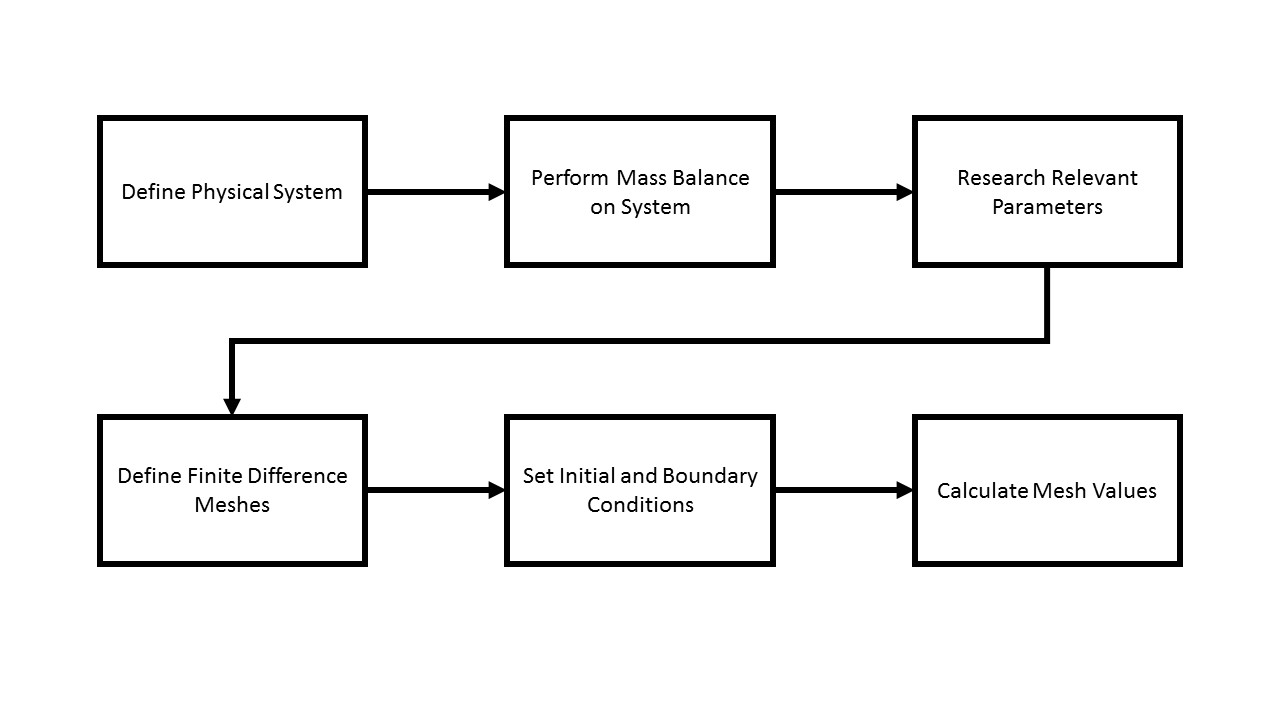
An analytical model using finite difference methodology was developed to predict performance of our phosphate uptake system over time. The methodology for developing the model is seen in Figure 1.

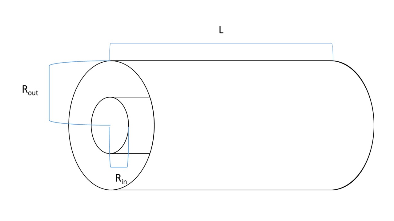
Figure 1: Overview of model development methodology. First, the physical system is defined, including physical parameters. Second, a mass balance is performed in each differential slice to develop an equation to describe the phosphate uptake rate. Third, relevant parameters, namely the instream phosphate concentration, are pulled from the literature. Fourth, the dimensions of the finite element meshes are defined and the meshes are created. Initial and boundary conditions are set before the meshes are analyzed using the finite difference equation.

The dimensions of the bioreactor were measured and are seen in Figure 2.

Figure 2: Schematic of the bioreactor system. Fluid flows into the outer annulus, where the encapsulated E. coli reside. The fluid reaches the far end of the cylinder and then flows out the central tube. R_in was measured as 3.1 cm, R_out as 3.8 cm, and L as 25.6 cm.

Mass Balances

Uptake rate in a differential volume during a differential time is modeled with Equation 1.

Where Cout is the extracellular phosphate concentration at position x and time t, C_in is the intracellular phosphate concentration at the same position x and time t, C_max is the maximum phosphate capacity of the cells, and k is the phosphate uptake constant. The phosphate uptake constant is a function of plasmid copy number, promoter strength, half-life of the phosphate uptake genes, and the diffusivity of the sol-gel matrix encapsulating the bacteria. For this model, k is assumed to be a constant value. Converting to finite difference form yields Equation 2.

Δt is a parameter of the model. The differential volume is calculated based off of the volumetric flow rate (Q) as seen in Equation 3.

This enables the creation of a mesh such that an entire differential volume is moved through over the course of the discrete time step. The maximum phosphate capacity of each differential volume slice is determined with cell density and maximum phosphate capacity per cell using Equation 4.

The cellular concentration is assumed to be 108 cfu/mL and the phosphate concentration per cell is assumed to be 4*10^-14 mol/cfu.

Two meshes are then defined: one to model phosphate concentration outside of the cells and one to model phosphate concentration within cells at all linear positions within the bioreactor at all time points for the length of the model (total running time is a preset parameter). The model is then run over the preset time parameter.

Assumptions

The model makes a few assumptions to simplify the calculations in order to build a general sense of system performance.

It is assumed cell growth over the time course of the model is negligible and therefore is not accounted for.
It is assumed flow velocity is the same at all radial positions in the reactor (perfect plug flow). Given that the width of the annuls is 0.7 cm and the flow rates are relatively low, the shear stresses are unlikely to create a large velocity gradient.
It is assumed that the uptake coefficient remains constant throughout all position and time points in the model. This assumption is valid because the genes are designed to be under constituitive control, resulting in a steady-state concentration of the membrane transport proteins.

Results

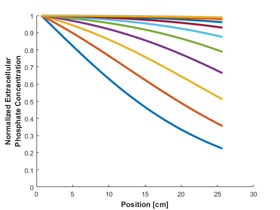
Concentration profiles of phosphate at various time points are seen in Figure 3.

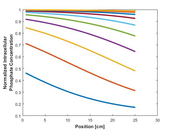
Figure 3: Concentration profiles of extracellular phosphate at equally-spaced time points in the model. The concentration is normalized to the instream concentration of phosphate. The profiles indicate a noticeable difference in uptake rates at various points in the reactor over time.

Similarly, concentration profiles across the reactor of phosphate within the cells are plotted in Figure 4.

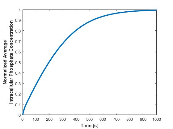
Figure 4: Concentration profiles of intracellular phosphate at equally-spaced time points in the model. The concentration is normalized to the instream concentration of phosphate.

Additionally, the average intracellular concentration of phosphate across all cells in the bioreactor is calculated and plotted against time (Figure 5).

Figure 5: Average intracellular phosphate across the entire bioreactor plotted over time. The concentration is normalized to the instream phosphate concentration. The plot shows the accumulation of phosphate of the entire bioreactor over time. As the concentration nears the maximum, the uptake rates slows and the reactor efficiency drops.

To determine the overall efficiency of the reactor, the exiting concentration of phosphate is divided by the original, instream concentration, and plotted against time in Figure 6.

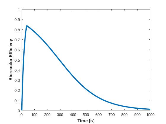
Figure 6: Bioreactor efficiency over time. The reactor peaks at 83.7% efficiency before decreasing as the cells near their phosphate capacity.

This plot embodies the usefulness of the model, as the reactor efficiency is a measure of system performance. The plot can be used to determine a cutoff point when the PAO should be replaced. For instance, if the cutoff efficiency is 50%, the filter would be replaced at the 300s mark, or every five minutes.

Effect of Varying Parameters

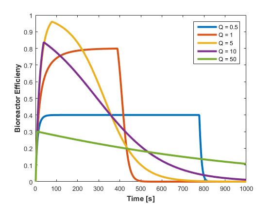
The effect of flow rate on the bioreactor was evaluated by simulating various flowrates (Figure 7).

Figure 7: Effect of flow rate on phosphate uptake over model simulation time. The model was run at various flow rates (0.5 mL/s, 1 mL/s, 5 mL/s, 10 mL/s, and 50 mL/s). The cells reach their maximum capacity of phosphate sooner as the flow rate slows.

The overall bioreactor efficiency was also calculated at various flow rates (Figure 8).

Figure 8: Bioreactor efficiency over time at various flow rates (0.5 mL/s, 1 mL/s, 5 mL/s, 10 mL/s, and 50 mL/s). For a replacement cutoff of 50% efficiency, a flow rate of 1 mL/s provides the longest lifetime of the reactor.

Conclusions

Preliminary modeling of the system has provided a general idea of the system performance and how often filters would have to be changed for effective operation. Future iterations of the model would rely on experimental data to get a more realistic value for k, the phosphate uptake coefficient. Future iterations could also inform the value of k further and explicitly define it as a function of plasmid copy number, promoter strength, and other factors.

MATLAB Code

clc
clear
close all

% Model Parameters
dt = 1; % [s]
flowRate = 10; % [mL/s]
RunningTime = 1000; % [s]
k = 5E-2; % [mL/s]
cellConc = 1E8; % [cfu/mL]

% Given values
length = 25.6; % [cm]
innerR = 3.1; % [cm]
outerR = 3.8; % [cm]
pPerCell = 4E-14; % maximum phosphate concentration per cell [g/cfu]
pMassConcIn = 5E-6; % initial phosphate concentration [g/mL]

% Constants
pMolarMass = 94.9714; % molar mass of orthophosphate [g/mol]

A = pi()*(outerR^2 - innerR^2); % annulus cross-sectional area [cm^2]
velocity = flowRate / A; % linear flow velocity [cm/s]
residenceTime = length / velocity; % residence time in bioreactor [s]

nt = RunningTime / dt; % number of time points in mesh
dl = velocity * dt; % width of finite volume [cm]
nl = floor(length / dl); % number of length points in mesh
dv = dl*A; % finite element volume [mL]

% multiply finite element volume by cell concentration to find cell count
% per volume
cellCount = dv * cellConc; % [cfu]
% determine maximum phosphate capacity per finite volume by multiplying
% phosphate capacity per cell by cell count
Pmax = pPerCell / pMolarMass * cellCount; % [mol Pi]

Cin = pMassConcIn / pMolarMass; % phosphate molarity of in stream [mol/mL]

% initialize meshes
Pout = zeros(nt,nl+1);
Pin = zeros(nt,nl);

% set initial and boundary conditions
Pout(1,:) = Cin; % initial condition: phosphate concentration is initial
Pout(:,1) = Cin; % boundary condition: all incoming concentration is initial

for t = 2:nt
for x = 2:nl+1
dP = k*Pout(t-1,x-1)*(1-Pin(t-1,x-1)/Pmax)*dt;
Pout(t,x) = Pout(t-1,x-1)-dP;
Pin(t,x-1) = Pin(t-1,x-1)+dP;
end
end

PinAve = zeros(nt,1);
for i = 1:nt
PinAve(i) = mean(Pin(i,:));
end

fontsize = 16;

figure(1)
plot(dt.*(1:nt),1-(Pout(:,nl+1))./Cin, 'LineWidth', 3);
ylabel('Bioreactor Efficieny','FontSize',fontsize,'FontWeight','bold');
xlabel('Time [s]','FontSize',fontsize,'FontWeight','bold'); axis([0 RunningTime 0 1]);
figure(2)
plot(dt.*(1:nt),PinAve./Pmax, 'LineWidth', 3);
ylabel({'Normalized Average', 'Intracellular Phosphate Concentration'},'FontSize',fontsize,'FontWeight','bold');
xlabel('Time [s]','FontSize',fontsize,'FontWeight','bold');
figure(3)
hold on
timepoints = 10;
timespace = nt / timepoints;
for i = 1:timepoints
plot(dl.*(1:nl+1),Pout(round(i*timespace),:)./Cin, 'LineWidth', 3);
hold on
end
ylabel({'Normalized Extracellular', 'Phosphate Concentration'},'FontSize',fontsize,'FontWeight','bold');
xlabel('Position [cm]','FontSize',fontsize,'FontWeight','bold');
axis([0 30 0 1]);
figure(4)
for i =1:timepoints
plot(dl.*(1:nl),Pin(round(i*timespace),:)./Pmax, 'LineWidth', 3);
hold on
end
ylabel({'Normalized Intracellular', 'Phosphate Concentration'},'FontSize',fontsize,'FontWeight','bold');
xlabel('Position [cm]','FontSize',fontsize,'FontWeight','bold');