Team:Newcastle/Model
Modelling
This page documents the dry lab experiments relating to our modelling.
ODE Modelling
As part of our work, we performed many different types of modelling, from rule-based modelling of our genetic parts to physics analysis of our microfluidics components. On this page, we discuss the ordinary differential equation (ODE) modelling of our components for use in a web-based ‘simulator’. We hope that our ‘simulator’ will demonstrate how our genetic constructs could fit into an electronic circuit.
Simulator Core
The core of our simulator features a set of ODEs that describe an abstract version of the transcriptional (Equation 1) and translational (Equation 2) processes in a cell.
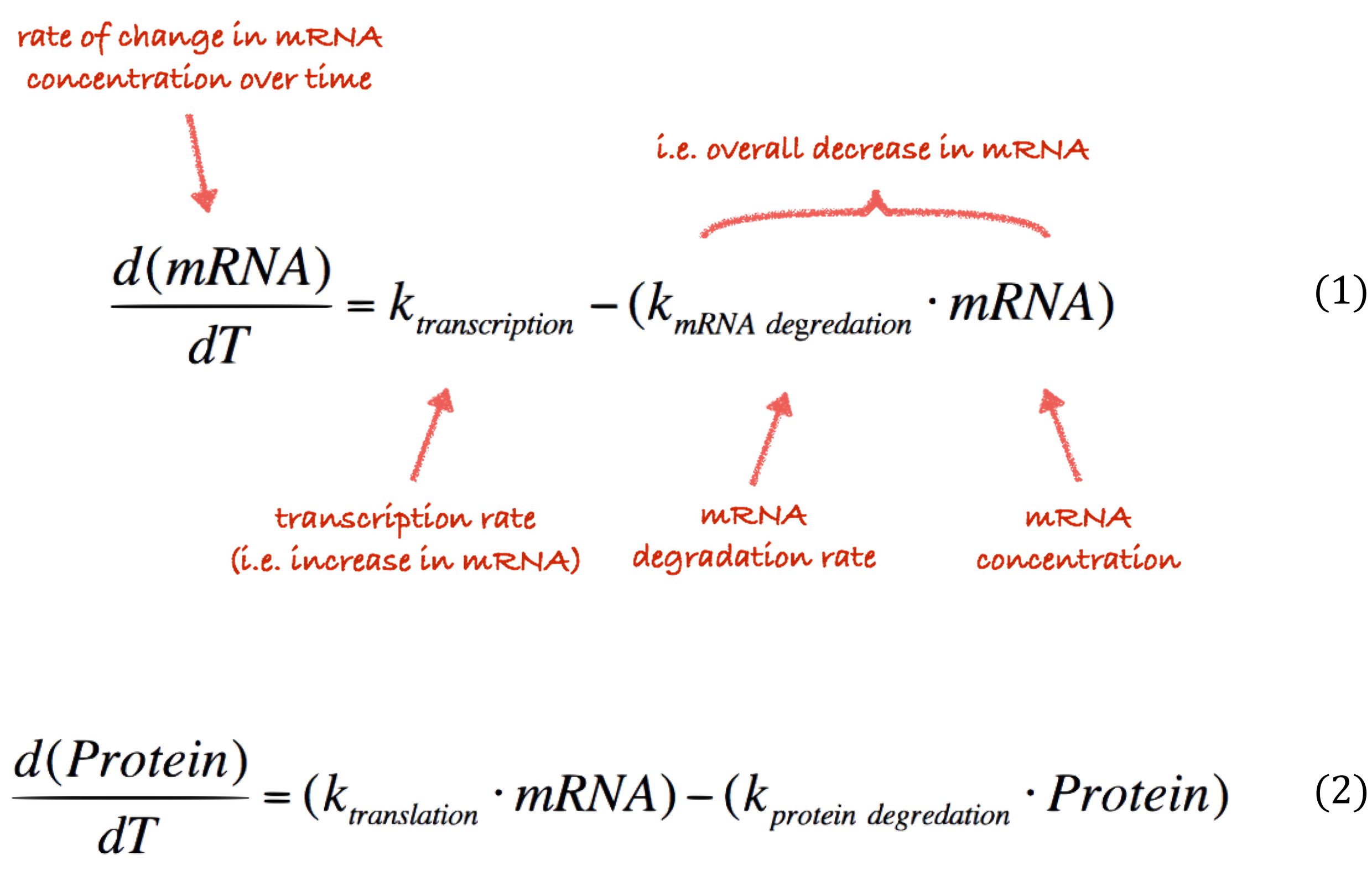
The rate at which these processes occur is controlled by a number of paramters, and . These constants describe the rate of transcription rate, degradation of mRNA, translation rate and protein degradation rate respectively. In our modelling we focus only on variation in the and parameters; we can fluctuate these values various promoter strengths and protein degradation tags. The other parameters are unrelated to any of the elements of our system that we control. Consequently, we have assigned these fixed values in our simulator.
Since our code is freely available, a modeller with different simulation requirements could easily change these parameters if they were meaningful in their scenario. We also constrain the other parameters in our simulator so that the simulation is stable when the user is given control over these values. For example, it might be logical for the user to select between a weak, medium or strong promoter. In this scenario, the user should not be required to know the exact numerical values of their choice. Although more advanced users may wish to be able to input their own values. For this reason, our simulation uses sane defaults for the transcription rate, , which is analogous to promoter strength.
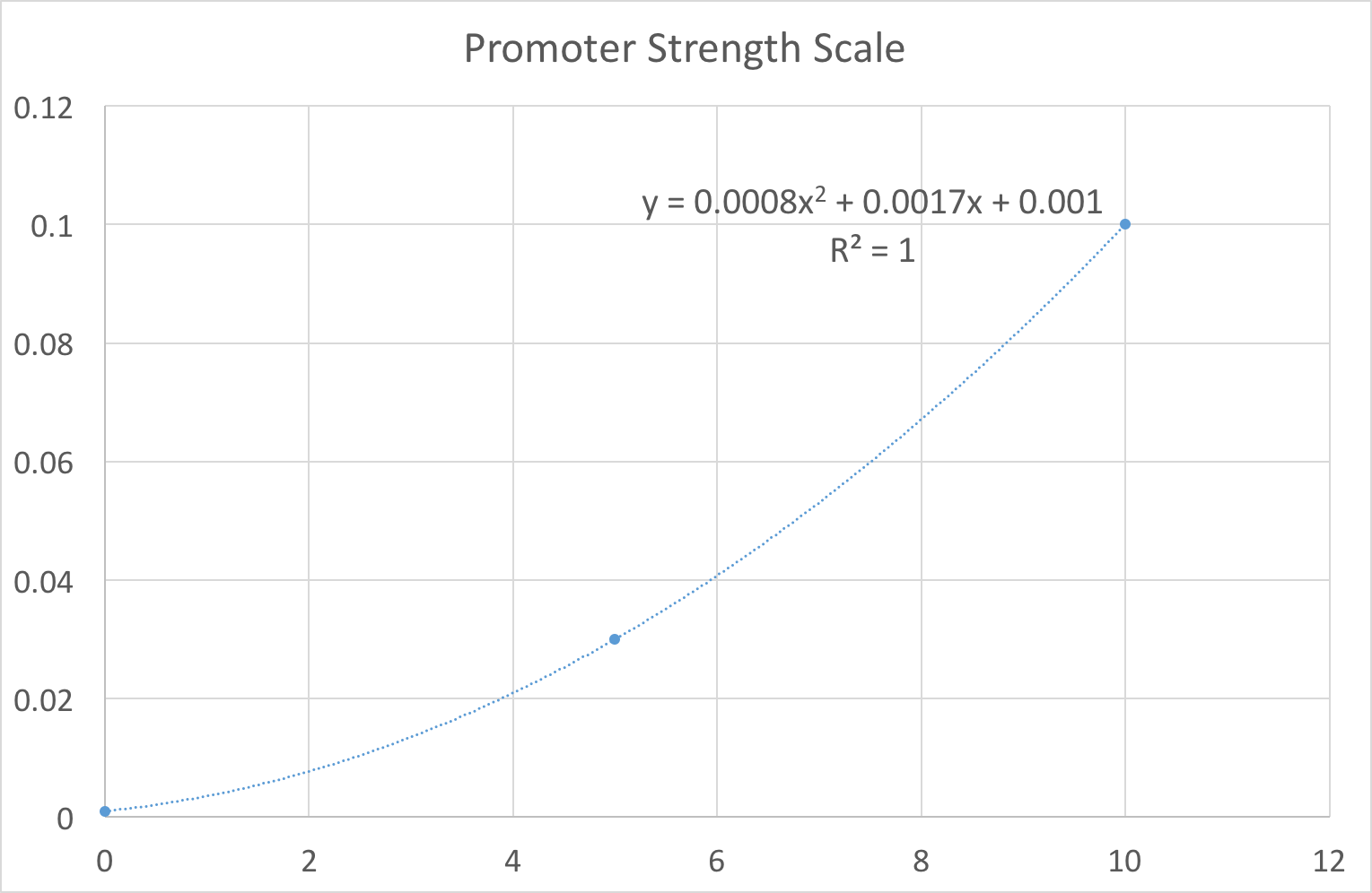
In our design work, users thought being constrained to these three options limited their ability to fully explore the biological system. For example, it would not allow the user to see the variation in gene product caused by slight noise in the promoter strength value, e.g. switching between 0.03 and 0.1 quickly. As our system is primarily a way of exploring the constructs we have built we wanted to limit the end user as much as possible. Therefore we set out plans to replace the notion of strong/medium/weak promoters with a more fine-grained scale. One that the user might control with a simple slider for example. To achieve this feat we fit our existing values using regression to a 10 point scale. This gave us an equation that we can use to map a user’s idea of ‘promoter strength’ to a transcription rate. As shown in Figure 1, the resulting equation was . Note that we deliberately ensured that to reflect the fact that there is always some background level transcription. In layman's terms, no biological promoter can be completely ‘switched off’.
The remainder of our simulator is built around these simple equations. The rest of this page will discuss how the other components were simulated using this technique and then integrated into the simulator. Our constructs were found to be easily adaptable to this form of model. However, it is not applicable in all situations. Our equations capture a simple ‘PRET’ (Promoter-Ribosome-Expression-Terminator) construct. As such it can be generalized to any number of protein expressions by having a tuple for each gene product in the model and separate counts of mRNA and protein.
Justification
We chose to build our simulator around a set of ODEs rather than using a more complex system that produced models in a format like CellML or SBML because it met our design goals. Primarily, this was ease of development and integration into the iGEM wiki system. Our main aim was to allow the simulator to be embedded in the wiki. In turn we felt that it was necessary to support the aims of the iGEM wiki system in preventing ‘bit-rot’, that is not having some aspects of our project hosted somewhere else where their uptime could not be guaranteed. This meant we needed a purely client side implementation and couldn’t ‘call out’ to other computers to perform the computation. When researching how we would construct our system we determined that the most straightforward of modelling our system in JavaScript without using any libraries or complex dependencies was to hard-code the ODEs.
Another aspect that makes the ODEs approach useful for us is that the level of abstraction they capture i.e., transcription and translation, corresponds directly with the level at which we design our BioBrick constructs. This makes it easy to translate between formats and allows for us to rapidly add new knowledge to the simulator as we develop our constructs. And vice versa, the simulations at this level translate directly to components in the system which we can control in our constructs. For example, we can directly influence the number of proteins in the cell by increasing the number of coding sequences on a construct. Whereas we can’t influence variables like the amount of free mRNA through our constructs alone.
There are some trade-offs to this approach. For instance, we lose access to tools that perform local and global sensitivity analysis, parameter estimation, etc., which limits the ‘depth’ of our models. We also lose out on interoperability with future software through interchange standards like SMBL. However, we believe that this doesn’t subtract from the quality of our models because their intended purpose is to encourage the user to think about the implications of interfacing bacteria with electronics rather than providing detailed models. In other words, our present systems are not complex enough to warrant modelling at a lower level of abstraction in the simulator.
That is not to say that we didn’t also perform lower level modelling. We also used rule-based modelling in the BioNetGen language using the RuleBender graphical tool. This allowed us to capture our systems in more detail and to ‘sanity check’ the simplified models we use here in our simulator.
Integration
There are a number of ways to integrate the differential equations presented above. The simplest is to iteratively compute the difference and add these to a ‘running total’ over the lifetime of the simulation. That is, for each time step compute where h is the step size, f is a differential equation such as those above. This method is known as Euler’s method. It can be visualised as fitting a series of straight lines to the given differential equation. It is, therefore, more accurate at small step sizes (the global error is proportional to the step size and the local error is proportional to the square of the step size). This is the method we use in our simulator.
 .
.
Zinc Uptake Model
Before adding our constructs to the simulator we first developed the models in MATLAB. Figure 2: This was done so that we could quickly get graphical output from our models and thereby assess their validity.
Our variable resistor works by varying the concentration of free zinc in an electrolyte in order to control the resistance. We wanted our model to reflect the zinc binding and release over time through the synthesis of SmtA, a metallothionein from Cyanobacteria. And to see the corresponding affect on the conductivity. For the electrolyte we chose to model this as zinc sulfate as this is a common electrolyte for which the conductivity data is well known (CRC Handbook of Chemistry, 1989). Because the conductivity is known for a variety of concentrations, we can relate this the number of free ions using the molecular weight of zinc sulfate (zinc sulfate decomposes to and in solution). We used the available data from the literature to fit an equation relating conductivity to the number of free zinc ions. We determined that this relationship was linear and takes the form . Where and are parameters found by our equation fitting ().
At time there is some amount of ions, in our model this is . Over time, SmtA is expressed and binds to these Zinc molecules, four ions per protein (Blindauer et al., 2002). Similarly, as the protein is degraded the zinc is released again and can participate in conduction. Our model is a simplified view of the system as it ignores cellular mechanics, like the rate of zinc transport into and out of the cell. Our model treats the system as free SmtA binding to free zinc, with the cell serving only as a producer of protein. This leads us to hypothesise that the cell is unnecessary, on the condition that SmtA remains stable outside of the cell.
From this observation we developed some additional variants of our variable resistor construct that would allow us to purify the SmtA and examine this question experimentally. We also investigated joining the SmtA protein to a LOV (light-oxygen-voltage) domain. LOV domains are found plant, fungi and bacterial proteins which participate in phototropism or circadian rhythm setting. All LOV proteins have a blue-light sensitive flavin chromophore which means they can be used as light sensitive switches in hybrid proteins. This has previously been explored as LovTAP (ETH Zurich iGEM, 2012 and Strickland et al., 2008). In our case we looked at using a LOV domain to create a light controlled zinc binding mechanism.
Modelling zinc binding requires a small extension to main ODEs used in our simulator. We came up with another ODE to model the amount of bound zinc.
The above equation is a variant of the protein production equation, , which captures that every time step, the free SmtA binds with some efficiency to the free zinc ions. This efficiency is modeled as the constant which is the percentage of the free proteins that bind each time step. Each protein that binds removes four zinc ions (we later chose to factor our this constant as a variable so that we could explore the impact that a better zinc binding protein would have). At the same time, some of the currently bound proteins are degraded, releasing four zinc ions each. This happens at the same rate as the protein degradation in the standard model.
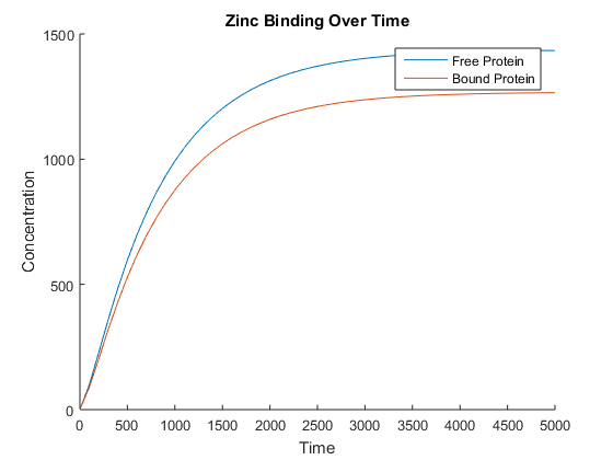
You’ll observe that at this point we’ve started to differentiate between bound and unbound proteins, but our model does not currently capture this. This inaccuracy prompted us to rethink our model, as by modelling the amount of bound zinc directly we had omitted an important biological process. This was most evident when we ran the model and found it to be unstable over large time steps (). While the bound zinc in this model followed an expected trend, closely following the amount of protein produced, it fluctuated between the trend and zero every 500 or so time steps. This was deemed undesirable, so we chose to adapt the model to include all intermediate steps of bound and unbound proteins. we achieved this feat using the same methodology to that of our original model that had zinc binding modelled directly.
The number of bound zinc ions can easily be found by multiplying the number of bound proteins by 4. This new model resulted in the expected behaviour, shown in Figure 3. Note that a larger time step was used to clearly show that the amount of free and bound protein diverge over time.
When we connected this with our conductivity model, however, we noticed that the conductivity was not affected. At this point we realised that to date, we had been modelling only a single cell when we need to be modelling populations of cells to see our desired effects on the correct scale.
For our zinc model this is a simple matter of multiplying the single cell model to reflect the behavior of a whole population. According to BioNumbers database there are approximately cells per ml in an overnight culture (Milo et al., 2010). As our chamber holds approximately 2 ml, we will use an estimated population size of of cells.
Using our population scale model we observe that the concentration of free zinc is not reduced enough to have any impact on the conductivity. We thought this might be a consequence of our model having too low protein expression, ~1400 proteins per cell. This would correspond to a cellular SmtA concentration of approx. 1.5 µM (according to BioNumbers, 1 µM corresponds to ~1000 proteins in Escherichia coli). We had difficulty finding protein expression quantified in this way as expression levels are usually determined using a reporter protein like GFP and the level given in arbitrary fluorescence units (e.g. Leveau et al., 2001). The best data we could find was on the concentration of CheZ in a typical cell, since this is a natural E. coli protein (with a role in chemotaxis) rather than an engineered expression system the values may not correspond well with our expression system. It is however suitable for modelling purposes. The concentration of CheZ in a typical cell is ~4-12 µM; this equates to between 4000 and 12000 proteins which is higher than the values we currently use in our model.
Assuming that eventually all of the proteins bind the zinc, our population can remove zinc ions from the solution. This calculation suggests that we should have less zinc in our solution, or a greater cell density. If we wanted to be able to remove all the zinc we would need to start with a solution. This corresponds to a conductivity of which represents a significant challenge to measure.
Because our model indicates limited success using this approach we used this feedback to explore other approaches to changing electrical conductivity. When we investigated alternative ways to change a mediums resistance we found that pH and conductivity (the reciprocal of resistivity) are intrinsically related. This is because pH is a measure of the number of H+ ions in solution and it is these ions, among others, that conduct current. The relationship between pH and H+ concentration is . Therefore, lower pH solutions have both a higher concentration of H+ ions and higher conductivity.
Altering the resistance in this way has the advantage that even if we were unable to measure resistance we knew we could still integrate this with electronics. We would be able to do this using readily available pH sensors which we knew about due to our discussions with Luis Ortiz at IWBDA 2016 who was working with this technique.
We adapted the basic genetic toggle switch design of Gardner et al. (2000) as shown in figure 4 by adding lacZ as the reporter (figure 5). When lacZ is expressed the E. coli can metabolise lactose in their growth media, this results in acid production which lowers the pH of the growth media and thereby also lowers the resistance.
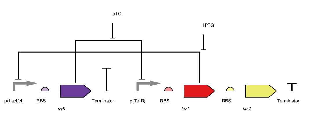
To toggle the expression of lacZ we chose a TetR/LacI scheme as this had been shown to be effective in previous iGEM projects like Wageningen 2014. In this scheme the addition of aTC to the medium inhibits the off signal (tetR expression) causing the on signal (lacI) and reporter to be expressed, this is the 'on' state. The addition of IPTG on the other hand causes the repression of the on signal (lacI), allowing expression of the off signal (tetR) which inhibits the further expression of the reporter. This is the off state. This two state system is shown in figure 5. In the future we wold like to further augment this design with a mechanism for reducing the pH in the off state, for example through Urease production. However this remains a challenge as the Urease protein is very complex (5 kb of DNA encoding 7 genes).
Biological Capacitor Model
As with all our models the biological capacitor is built around the core equations for transcription and translation. For our biological capacitor the only extension upon our existing model base is that instead of keeping track of one protein we have to keep track of three: lambda repressor, 434 repressor, and a reporter protein. In our construct, we chose GFP as our reporter gene. However, in the final construct, this protein would ideally be the protein that causes the capacitor to charge so that they could be chained together. The following set of ODEs mathematically describe the system:
Since our construct contains twice as many coding sequences for 434 repressor as lambda repressor its concentration increases twice as fast which is reflected in the above equations. By virtue of it growing twice as fast, it also degrades twice as fast because of the equations above. This is the desired behaviour since in our construct we use a ssRA degradation tag to have the 434 repressor degrade faster. In reality it may not be the case that the degradation tag results in a 2x speed up in degradation but this can be accomodated in the model. We would do this by having seperate translational constants such that and where captures the relative degradation ratio of lambda to 434 repressor and could be determined experimentally.
Our biological capacitor was constructed to mimic the behaviour of an electrical capacitor. Rather than accumulating charge, the capacitor accumulates proteins that are used to drive an output when the input signal stops being applied. For demonstrative purposes of showing we can partially mimic this behaviour, we assume that the signal is applied constitutively and then switched off by the addition of a chemical. In our construct this is L-arabinose, but from a modelling perspective, all that needs to change is the promoter strength.
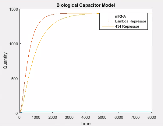
As with our previous models, there are transcription and translation rate constants that directly control the amount of protein synthesised. By using the same strong promoter values as in our other models, we get the standard behaviour. Namely, that the number of proteins in the cell gradually increases up to some carrying capacity at which point they degrade at the same rate as they are produced and the amount of protein in the cell levels off.
A simulation that simply accumulates proteins is not of significant biological interest. Thus we needed a way to model the addition of our repressor L-arabinose. We observed that fundamentally, inducers and repressors alter the promoter strength. Since there will always be leaky constitutive production, the addition of an inducer simple increases the strength, and the addition of a repressor decreases the strength of the promoter.
In our model because 434 and lambda repressor are under the control of the same promoter they effectively share a transcripton rate which corresponds to the strength of that promoter. Consequently to simulate the addition of a repressor in our model we need only vary the value of this transcriptional constant. Figure 6 shows the behaviour of the system when the promoter is weakened at . We changed the promoter from strong to weak using the values outlined in the ‘simulator core’ section.
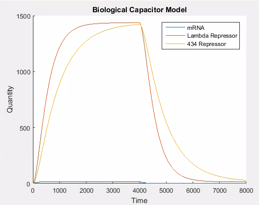
As can be seen in Figure 7, the 434 repressor quickly decays to the point where there is more lambda repressor than 434 repressor. At this stage, we would expect our output protein to be produced as 434 repressor would out compete lambda repressor and prevent transcription of the output protein.
We tried different approaches to modelling this change. Our first method used a stochastic approach. This approach modelled the competition between lambda repressor and 434 repressor to induce/repress production (i.e. transcription and translation) of our output protein. In this variant of the model we used a ‘lottery’ system to decide the transcriptional rate of the output protein. For each time step, if the 434 repressor ‘won’, then the promoter is ‘weak’; otherwise the promoter is ‘strong’. The way the lottery system works is that each protein is given a number of ‘tickets’ in direct proportion to the total amount of protein that exists. A ticket is then chosen at random and if it belongs to 434 repressor, then it ‘wins’, otherwise lambda wins. This can easily be simulated using the proportion of each protein to allocate tickets on the line 0-1 and then using a random number from 0 to 1 to determine the winner. This results in the following behaviour in the system.
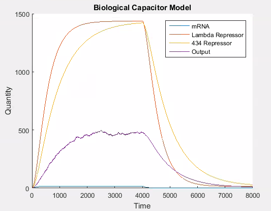
As can be seen in Figure 6, the stochastic model results in leaky behaviour. This type of behaviour was not the intended behaviour of our construct. The output signal follows the same trend as the lambda and 434 repressor, but with a large amount of noise. In our construct, we would expect that the expression of the output signal would remain low until the amount of 434 repressor was greater than the amount of lambda repressor at which point there would be a spike in the output signal which would decay as the repressors do. We think that this is similar to having the promoter for the output be ‘weak’, while having it be ‘strong’ when there is more 434 than lambda repressor. It is easy to adapt the model to this behaviour, as this is the same technique we use to model the addition of L-arabinose.
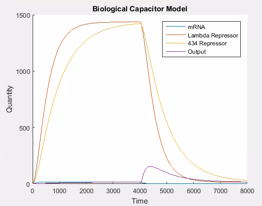
Figure 7 shows the desired behaviour of our system, which confirms that our construct needs to work as described above to exhibit the correct behaviour. If on the other hand, the interaction between the lambda and 434 repressor behaves as in the stochastic simulation then our construct will not work as expected. Although we expect our construct to behave as in this latter simulation we will need to verify this empirically.
Circuit Analysis
Because our components are to be integrated into electrical circuits, we needed a way of modelling how their resistances would affect other circuit components as well as a means of determining the current though, and voltage across, each of the components as this effects the heat dissipated in the component as a result of the Joule effect.
After some research we settled on using ‘analysis by superposition’ as our circuit analysis technique. This allows us to have multiple voltage sources in our circuit which is important as we want to be able to mix microbial fuel cell sources and standard DC sources like batteries and see the effect. Circuit analysis by superposition considers each voltage source at a time (‘shorting’ out the others) and then summing the resulting voltage values to get the final voltage drop for all components.
Before we could perform our analysis we needed to decide on our representation of our circuits. For our components, we have chosen to consider our systems as a series of resistors and sources, grounded at either end. This creates a linear circuit like the figure below.

Computationally we build our circuits as linked lists for easy traversal and simple editing operations. Additionally, the node structure of the linked list allows the system to generalise to parallel circuits, which would be represented by a graph data structure if at a later date we choose to implement this functionality.
The algorithm for analysing such circuits is simple, and is illustrated in the worked example below.
Circuit Analysis Example
Consider the circuit shown here.

Step 1: Short each voltage source in turn and compute the voltage across the resistors.
Shorting the 1.5V source leaves only the 9V source, the voltage across each resistor can then be found using the voltage divider formula: .
Therefore for R1 we have, . And for R2 we have, .
We can check our answers make sense by seeing that they sum to , ✓.
Shorting the 9V source leaves the 1.5V source. The voltage across R1 is . Note that the voltage is positive even though the source is after the resistor because it is ‘dragging up’ the ground. Across R2 the resistance is .
Step 2: Sum the total voltage across each resistor.
For R1 the total voltage drop is and for R2 it is . Again we can check that our total voltage drop matches the voltage supplied in the circuit, ✓.
Step 3: Finally we can derive any of the other data we need using the voltage drop through each component along with other equations. For example we can compute the current using Ohm’s law, . That is, the current through R1 is and through R2 is . As you would expect the current is the same all the way through the circuit.
We checked this analysis by modelling the same circuit in an existing circuit simulator as shown here, where we got the same results.
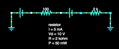
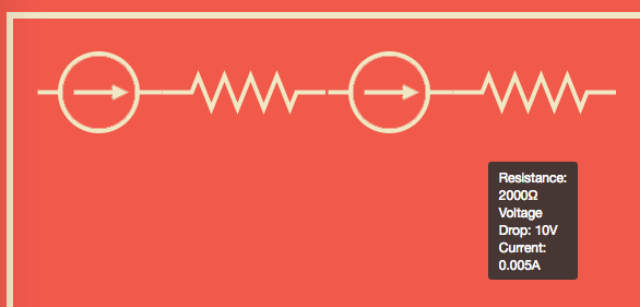
You can also see the same circuit in our very own simulator implementing this technique.
Multiphysics Modelling
We used multiphysics modelling through the COMSOL software to inform the design of our physical hardware. When we began our modelling we wanted to assess the effect of joule heating on various fluids. This was important to us as we wanted to trigger the E. Coli heat shock response using this effect. The joule effect is the heating caused when power is dissipated in a resistor. For us the resistive material is the bacterial growth medium. Whilst the power dissipated in a resistor can be computed easily from Ohm's law the actual temperature change is determined by a large number of variables. For instance, the specific heat capacity of the material, the surface area exposed to cooling, the temperature gradient between the material and the surrounding air, or another material. It is for this reason that we chose to use multiphysics modelling in our design work.
We created models of the geometry of various containers we had available to use in our lab and then began investigating the physical properties of bacterial growth media. At this point we had to call upon the assistance of another iGEM team, team Exeter to help determine the specific heat capacity of different growth media such as M9 and LB as we did not have the equipment available to conduct the studies ourselves. Onve armed with this information and the physical properties of our container materials which could be found in the COMSOL library we were able to model the temperature change in growth media. This initial modelling told us that it was indeed possible to get our desired temperature change of 10°C from the joule effect.
Developing our multiphysics model further we were able to establish which voltages and currents would cause our desired temperature change. We found that for our original containers the required voltage was far too high, on the order of 100V. This would limit the use of our technology to places where this volunteer could be produced safely. This is counter to our goal as a foundational advance team to enable as many people as possible to explore our technology.
Because we had developed a model we were able to alter the parameters and see if we could reduce the required voltage. We set a target of 30V as this can be safely produced in the lab using the bench top power supplies usually used for running gel electrophoresis experiments.
Or modelling told us that to achieve our 30V goal we would have to switch to a micofluidics scale. This is largely due to the fact that bacterial growth media are largely water, which has a high specific heat capacity which makes it good for cooling applications but not so good for heating. Directly following this modelling we designed custom geometries for micofluidics chambers that we went on to fabricate. Or modelling having a direct impact on our design work.
Temperature Change
As some of our parts are based on exploiting the the heat-shock response of E. coli it is important that we be able to determine the temperature change over time for our components. Using what we learnt in our physics modelling using COMSOL we knew we could approximate the temperature rise from the Joule heating effect using the power dissipated in the component and the thermal conductivity of the media (which we determined with the help of the Exeter iGEM team).
For our models we use and . Where K is the thermal conductivity (for LB broth this is ), L is the length and A is the area of the container.
We also looked at using where and is the specfic heat capacity, which we know for LB is similar to water (). Both of these equations give similar order of magnitude approximations. Unfortunately they are not complex enough to capture aspects liek the cooling effect of the surrounding air on the components which limites the accuracy of our model somewhat and can lead to incorrect data in the simulator.

Given more time we would have tried to include some of these aspects in our simulator or found a way to include data from external programs like COMSOL which we were able to use to perform this more sophisticated analysis.
The UI
We chose to build a UI for our models using HTML so that other people could explore the ways our technology would work in an easy way. Ideally, through our iGEM wiki. This is an important part of being a foundational advance team, showing how our technologies could be used.
To speed up development our UI was constructed around the existing JavaScript models, which we ported from the above MATLAB models and tied to an integrator which is always running in the background. We used a number of libraries to aid our development, including jQuery UI to allow for drag and drop circuit construction, the Spectre.css CSS framework for basic page layout and, Chart.js to show the output from our models.

You can try out more circuits in our editor to see the effect of using a bacterial resistor among other things.
References
- Blindauer, C. A., Harrison, M. D., Robinson, A. K., Parkinson, J. A., Bowness, P. W., Sadler, P. J. and Robinson, N. J. (2002), Multiple bacteria encode metallothioneins and SmtA-like zinc fingers. Molecular Microbiology, 45: 1421–1432. doi:10.1046/j.1365-2958.2002.03109.x
- Gardner, T.S., Cantor, C.R. and Collins, J.J., 2000. Construction of a genetic toggle switch in Escherichia coli. Nature, 403(6767), pp.339-342.
- Leveau, J.H. and Lindow, S.E., 2001. Predictive and interpretive simulation of green fluorescent protein expression in reporter bacteria. Journal of bacteriology, 183(23), pp.6752-6762.
- Milo, R., Jorgensen, P., Moran, U., Weber, G. and Springer, M., 2010. BioNumbers—the database of key numbers in molecular and cell biology. Nucleic acids research, 38(suppl 1), pp.D750-D753.
- Strickland, D., Moffat, K. and Sosnick, T.R., 2008. Light-activated DNA binding in a designed allosteric protein. Proceedings of the National Academy of Sciences, 105(31), pp.10709-10714.