Team:ShanghaiTechChina B/Model

Model

This summer, we were trying to tracing abnormally high NO concentration in people's guts. We want to simulate NO distribution in our bowels through modeling. We turn to the discussion of time-dependent diffusion processes, where we are interested in the spreading and distributing of NO with time.

Diffusion Equation

The equation for the rate of change of the concentration of particles in an inhomogeneous region, diffusion equation, also called 'Fick's second law of diffusion', which in this case relates the rate of change of NO concentration at a point to the spatial variation of the NO concentration at that point:$$\frac{\partial c}{\partial t}=D\frac{\partial ^{2}c}{\partial x^{2}}$$

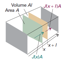
Figure 1. The net flux in a region is the difference between the flux entering fromthe region of high concentration (on the left) and the flux leaving to the region of low concentration (on the right). (Reference: P W Atkins. Atkins’ Physical chemistry, 7th Ed., Oxford: Oxford University Press, 2002, 776)

Justification

Consider a thin slab of cross-sectional area A that extends from x to x+l.

Let the NO concentration at x be c at the time t. The amount (number of moles) of particles that enter the slab in the infinitesimal interval dt is JAdt, so the rate of increase in molar NO concentration inside the slab (which has volume Al) on account of the flux from the left is$$\frac{\partial c}{\partial t}=\frac{JA\mathrm{d}t}{Al\mathrm{d}t}=\frac{J}{l}$$

There is also an outflow through the right-hand window. The flux through that window is J′, and the rate of change of NO concentration that results is$$\frac{\partial c}{\partial t}=-\frac{J'A\mathrm{d}t}{Al\mathrm{d}t}=-\frac{J'}{l}$$

The net rate of change of NO concentration is therefore$$\frac{\partial c}{\partial t}=\frac{J-J'}{l}$$

Each flux is proportional to the NO concentration gradient at the window. So, by using Fick's first law, we can write$$J-J'=-D\frac{\partial c}{\partial x}+D\frac{\partial c'}{\partial x}=-D\frac{\partial c}{\partial x}+D\frac{\partial}{\partial x}\left[c+\frac{\partial c}{\partial x}l \right]=Dl\frac{{\partial}^{2}c}{\partial {x}^{2}}$$

The viscosity of water is 0.891 cP (or 8.91 × 10^-4kg·m^-1·^-1), and the effective radius of NO approaches 0.36 nm in this case.

Diffusion Coefficient

With the constant D,which is called the diffusion coefficient, to be obtained, the formula above cannot be solved.

The following picture shows the flux of particles down a concentration gradient. Fick’s first law states that the flux of matter (the number of particles passing through an imaginary window in a given interval divided by the area of the window and the duration of the interval) is proportional to the density gradient at that point. $$J(\mathrm{matter})=-D\frac{\mathrm{d}\mathcal{N}}{\mathrm{d}z}$$

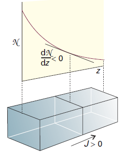
Figure 2. The flux of particles down a concentration gradient. Fick’s first law states that the flux of matter (the number of particles passing through an imaginary window in a given interval divided by the area of the window and the duration of the interval) is proportional to the density gradient at that point. (Reference: P W Atkins. Atkins’ Physical chemistry, 7th Ed., Oxford: Oxford University Press, 2002, 757)

If we divide both sides of this equation by Avogadro’s constant, thereby converting numbers into amounts (numbers of moles), then Fick’s law becomes$$J=-D\frac{\mathrm{d}c}{\mathrm{d}x}$$

In this expression, D is the diffusion coefficient and dc/dx is the slope of the molar concentration. We can obtain NO's diffusion coefficient in water either by experiments or by calculations. Finally we choose to do the calculations.

For dilute non-electrolyte A, its diffusion coefficient in solvent B (also called the infinite-dilute diffusion coefficient) can be estimated by Wilke-Chang equation:$${D}_{AB}=7.4\times {10}^{-15}\frac{{(\Phi {M}_{B})}^{T}T}{\mu {{V}_{A}}^{0.6}}\mathrm{{m}^{2}/s}$$

In the equation,

D_AB — The inter-diffusion coefficient in an infinitely-dilute solution, m²/s.
T — The temperature of the solution, K. In our case, it is 0.5.
μ — The viscosity of B, Pa·s.
M_B — The molar mass of B, kg/mol.
Φ — The parameter of association of solvent. (Introduction of the association parameter into the formula is brought about by the fact that associated molecules behave like large-size molecules and diffuse at a lower rate; the degree of association varying with mixture composition and with molecule types. Therefore, Wilke and Chang presented the values for most widespread solvents: for water φ=2.6; methanol, 1.9; ethanol, 1.5; benzene, ester, heptane and non-associated solvents, 1.)
V_A — The molar volume of solute A at a boiling point under normal conditions, cm³. It can be estimated by Tyn-Calus Method: V=0.285V^1.048, while V_c is the critical volume of a substance and measures 57.7 for NO.

Results

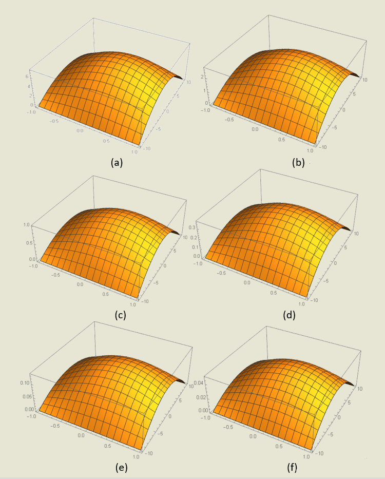
Figure 3. NO concentration distribution with time around the wound.

The six pictures demonstrate the NO concentration distribution with time (with the 1 s interval) around the wound caused by IBD. The concentration is shown along the Z-axis (unit: D). The intestinal lies along the X-axis (unit: 5 mm, Y-axis the same) with intestinal walls surrounding it. To simplify the situation, we assume that the dissipative NO molecules gathered altogether as a dot at time 0 which is located on the lower part of the intestinal walls, and the walls consume all the NO molecules within its range.

For loads of assumptions and approximations are used, this model still needs refined conditions to approach the fact. However, it has simulated the characteristic of NO diffusion in the intestinal and provides us with some information on detection of NO concentration from the calculation point of view.