Team:TAS Taipei/Model
Model
Cataract prevention occurs over 50 years, so we cannot perform experiments directly on the long-term impact of adding GSR or CH25H. Computational biology allows us to predict cataract development in the long-term. These models allow our team to: (1) understand the impact of adding GSR-loaded nanoparticles into the lens over a 50 year period and (2) design a full treatment plan on how to prevent and treat cataracts with our project. Therefore, the results of our model are essential in developing a functional prototype.
For clarity, we will discuss each model in detail with respect to prevention (using GSR) only. At the end, we extend these results to treatment. In addition, we include collapsibles for interested readers and judges, in order to fully document our modeling work (eg. assumptions, mathematics, and full analysis) while keeping the main page clear with basic points only.
If you are interested in the programming/source codes of these computational models, please contact Avery Wang, at averyw17113532@tas.tw or averyw09521@gmail.com.

Introduction
Guiding Questions
How much GSR to maintain in the lens? (GSR Function)
How to maintain that amount of GSR using nanoparticles and eyedrops? (Delivery Prototype)
Focus of Models
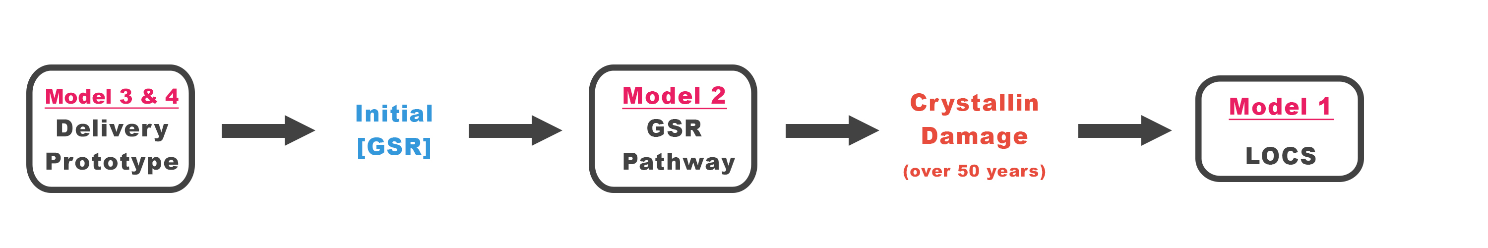
Since our construct is not directly placed into the eyes, how our synthesized protein impacts the eye after it is separately transported into the lens is of greater importance. As a result, we create models with the intent on understanding how GSR and CH25H impacts the eye, and how we can control its impact with a well-designed delivery prototype.
Prevention: GSR Function
Model 1: Crystallin Damage
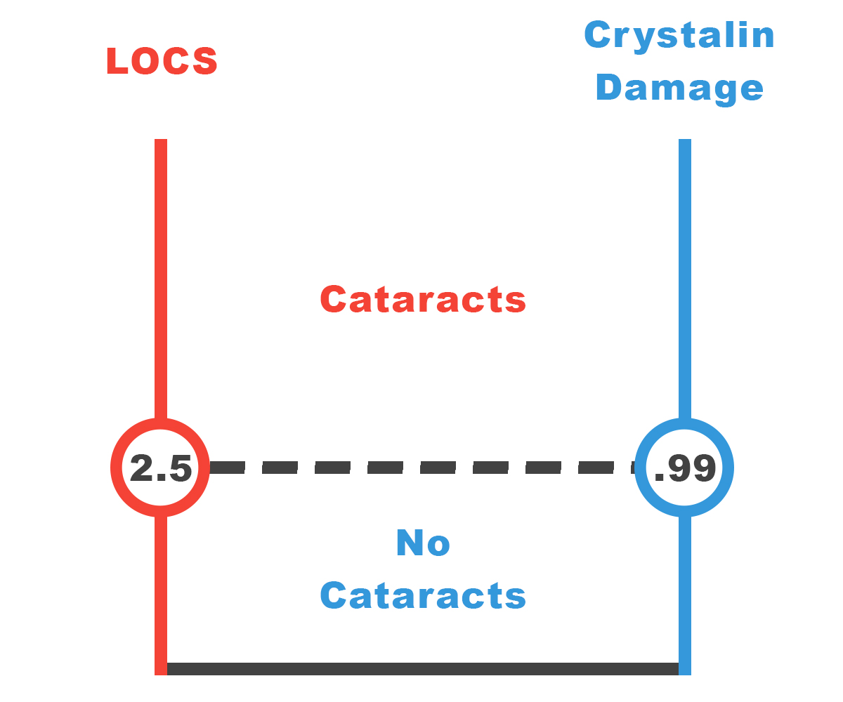
The amount of damage to crystallin by H2O2 determines the severity of a cataract (Spector 1993). We relate the amount of crystallin damage to the corresponding rating on the LOCS scale, used by physicians to rate cataract severity. Our goal is to lower LOCS to below 2.5, the threshold for surgery. Through literature research as well as our own experimental data, we find the maximum allowable crystallin damage to prevent a LOCS 2.5 cataract from developing.
Measurement of Cataract Severity
There are three ways of measuring cataract severity, each used for a different purpose.
- Lens Optical Cataract Scale (LOCS): Physicians use this scale, from 0 – 6, to grade the severity of cataracts (Domínguez-Vicent 2016).
- Absorbance at 397.5 nm: This is the experimental method, used by our team in the lab (c.d.)
- Crystallin Damage: This is a chemical definition. We quantify cataract severity as a function of how much oxidizing agents there are, as well as how long crystallin is exposed to oxidizing agents. (Cui X.L. 1993)
LOCS to Absorbance: Literature Data
Numerous studies show how absorbance measurements can be converted to the LOC scale that physicians use. With the results of Chylack, we construct the first two columns in Table 1 (Chylack 1993).
Absorbance Equivalence to Crystallin Damage: Experimental Data
We use experimental measurements from our team’s Cataract Lens Model (Link). They induced an amount of crystallin damage, and measured the resulting absorbance. The experimental results are listed in Table A, and Figure 4.A, we calculate the equivalent crystallin damage of each LOCS rating and absorbance, and create the third column of Table 1.
| LOCS | Absorbance (@397.5 nm abs units) |
Crystallin Damage (M-h) |
|---|---|---|
| 0.0 | 0.0000 | 0.0000 |
| 0.5 | 0.0143 | 0.1243 |
| 1.0 | 0.0299 | 0.2878 |
| 1.5 | 0.0497 | 0.4697 |
| 2.0 | 0.0751 | 0.6949 |
| 2.5 | 0.1076 | 0.9883 |
| 3.0 | 0.1492 | 1.3747 |
| 4.0 | 0.2706 | 2.5259 |
| 5.0 | 0.4691 | 4.3472 |
Conclusion
To guarantee that surgery is not needed for 50 years, we need to limit crystallin damage to 0.9883 units. If crystallin damage goes above this threshold, then surgery is needed. This is the crystallin damage threshold for a LOCS 2.5 cataract.
Motivation
Crystallin damage is the chemically significant way to quantify cataract severity (Cui X.L. 1993). Physicians grade cataracts on a LOCS scale from 0 to 6, with 2.5 usually being the threshold for surgery. This standard method to determine cataract severity is through optical analysis, which is not applicable for chemical analysis. (Chylack)
The purpose of this model is simple. In Model 2, we find the amount of GSR to maintain in order to ensure a cataract remains below a certain severity. Before we can do that, we must find a way to relate the physical definition of cataract severity (LOCS) to the chemical definition (crystallin damage) in Model 1.
We use literature data to relate LOCS to absorbance, which is still a physical property, but is frequently used in the lab. Then, with experimental data, we relate crystallin damage to absorbance, thus completing the link between the chemical and the physical definitions.
Quantification of Crystallin Damage
Crystallin damage is difficult to quantify, as few literature sources attempt to quantify it. We propose a mathematical way to measure crystallin damage based on how complete the degradation reaction of crystallin is complete depending on the amount of H2O2.
Crystallin damage depends on two factors: (1) the amount of H2O2 crystallin is exposed to, and (2) the time crystallin is exposed to H2O2. Therefore, we can mathematically quantify this by integrating the amount of H2O2 in the crystallin over time: \[c.d.(t) = \int_{0}^{\infty} [H_2O_2]_t dt\]
We define one unit of crystallin damage to be the equivalent damage caused by exposing the amount of crystallin in the human eyes 1 M of H2O2 for 1 hour, with units M-h. We make an assumption here, described fully in “Assumptions” #1.
Note that 1 M-h is a significant amount of crystallin damage, because the concentration of crystallin in the eyes is extremely small, in the neighborhood of 10 uM (Fraunfelder 2008). In addition, the eyes have a naturally occurring antioxidant system that lowers the concentration of H2O2, so it will take much longer than an hour of exposure until 1 M-h of crystallin damage is reached.
Data Analysis
Using Experimental Data for Model
In each trial (see Data Documentation), we added H2O2 of a known concentration to fish lens, and allowed crystallin to degrade for some set time. With all four assumptions, we can calculate the theoretical crystallin damage that occurred. Meanwhile, experimentally we found the absorbance of the degraded crystallin. We find a link between crystallin damage and absorbance.

Model Adjustment
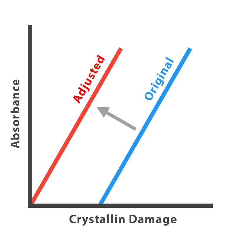
When determining the relationship between absorbance and crystallin, in Figure 4.A the best fit line has a x – intercept that is nonzero. However, when converting each absorbance rating to equivalent crystallin damage in Table 1, we ignore the constant term. When doing the experiments, the fish lens may have contained GSH that is still active, so the fact that the crystallin is exposed to H2O2, the degradation reaction does not happen until all GSH is depleted, and crystallin damage begins to form. We subtract around 1 unit of crystallin damage from all values, as shown in Figure 4.B.
Model 2: GSR Pathway
Now that we know how much we need to limit crystallin damage to LOCS 2.5, we model the naturally occurring GSR Pathway in the lens of a human eye. We calculate the necessary GSR concentration to be maintained over 50 years so that the resulting cataract is below LOCS 2.5.
Chemical Kinetics Model: Differential Equations
By various enzyme kinetics laws, fully documented in the collapsible, we build a system of 10 differential equations based on 6 chemical reactions (Ault 1974, Pi 2004). All parameters, constants (Table B), and initial conditions (Table C) are based off literature data (Ng 2007, Melissa 2012, Saravanakumar 2015, Salvador 2005, Adimora 2010, Jones 2008, Martinovich 2005). Estimates made are also shown with assumptions and reasoning. The details are shown in the collapsible for interested readers.
Blackbox Approach: Testing GSR Impact
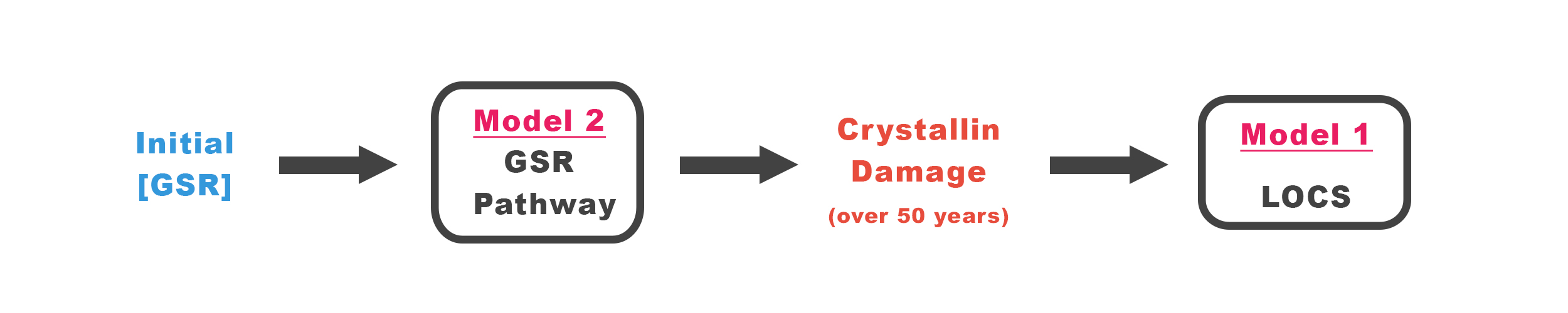
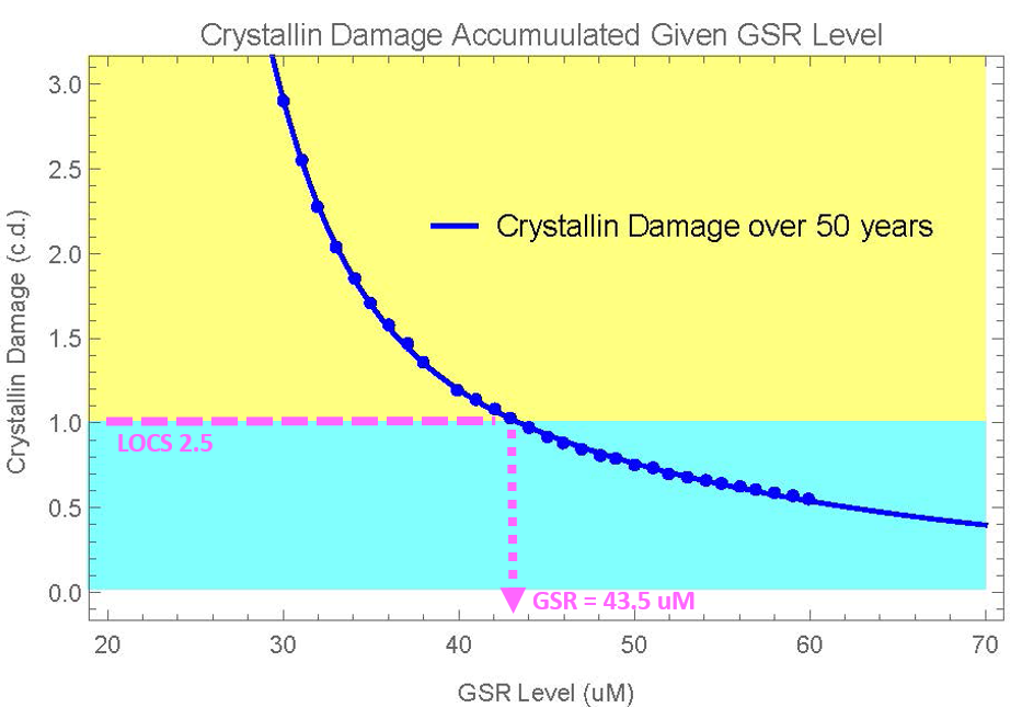
Our modeling approach is seen in Figure 4.2, where vary the input, Initial GSR concentration, holding all other variables constant, and numerically solve for the amount of hydrogen peroxide over time. We can find the amount of crystallin damage accumulated over 50 years if different levels of GSR is maintained, which we graph in Figure 4.3.
From this graph, we can find the GSR concentration needed for the LOCS 2.5 threshold.
Crystallin Damage vs. GSR Level
According to literature data and our model, the naturally occurring GSR concentration is 10 uM (Fraunfelder 2008). All curves show crystallin damage decreasing as GSR levels are increased, which supports both research and experimental data, and suggests that this prototype is effective in preventing crystallin damage. However, GSR levels need to be raised significantly, up to 40+ uM from the natural 10 uM of GSR in order to show long-term protection.
Figure 4.3 shows the amount of GSR we need to maintain for 50 years in order to prevent a LOCS cataract of a certain severity. The row of interest is LOCS 2.5, the threshold for surgery. Notice that we say “maintain” the level of GSR. This level needs to be constant at all times for 50 years for full prevention. The delivery of GSR to maintain this level is discussed in Model 3.
Conclusion
We need to maintain (NOT add) 43.5 uM of GSR in the lens so that the crystallin damage recorded over 50 years is below the LOCS 2.5 threshold.
Prevention: Prototype Function
Model 3: Nanoparticle Protein Delivery
To maximize delivery efficiency to the lens, we encapsulate GSR in chitosan nanoparticles (Wang 2011, Tajmir-Riahi 2014). From Models 1-2, we have found the necessary concentration of GSR that needs to be maintained in the lens. Now we design nanoparticles that will maintain those amounts. We build a model find how nanoparticles release GSR at appropriate rates to control the amount of GSR in the lens, and find the best engineered design for nanoparticles.
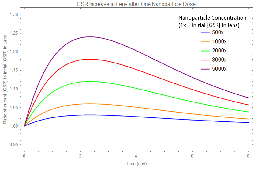
Single Dose: Change in GSR Concentration
In finding the best engineered design, we take into account variables such as nanoparticle radius and concentration. We build a differential equation model for the impact of a single dose of nanoparticles over time. To generalize the model, instead of using absolute concentrations, we use relative concentration, with respect to the natural amount, or initial amount of GSR in the lens. The full mathematics and details can be found in the collapsible.
We get two curves, the concentration of GSR outside nanoparticles subjected to degradation (Figure 4.4), and the release of GSR from nanoparticles (Figure 4.5), over time. This allows us to predict nanoparticle delivery rates before we perform the actual experiments (Link)
Comparison with Experimental Data
Yet in our model, we do not know the thickness of the nanoparticle diffusion layer. After performing experiments, we can use measurements of our prototype device to find this thickness, and refine our model. A direct comparison of our model with our experiment data is shown in Figure 4.5.

Multiple Dose: Change in GSR Concentration
Each dose of nanoparticles, represented in the Single Dose model, can be repeated to create the Multiple Dose model. Below is a graph of GSR concentration over time when multiple doses of nanoparticles are added.
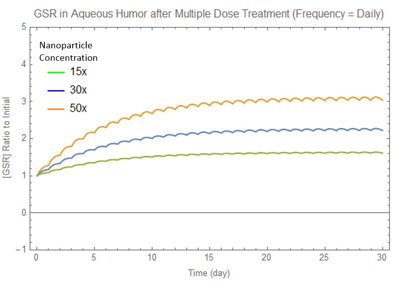
In Figure 4.6, all curves approach equilibrium, after which the concentration oscillates about equilibrium. We have three goals, in order of importance for best nanoparticle design:
- GSR equilibrium concentration equal to amount we desire (i.e. 43.5 uM from Model 2)
- Stability of concentration at equilibrium (Model 4 goes into deeper depth regarding sensitivity)
- Time to reach equilibrium (time for full prevention to come into effect)
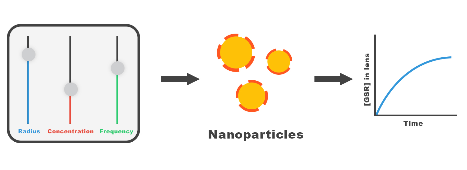
To do so, we can alter different variables: GSR concentration in nanoparticles, nanoparticle radius, and dose frequency. For a full analysis of how each variable impacts the concentration function, see the collapsible. Below is a summary of the results:
| Independent Variable | Time to Reach Equilibrium | Equilibrium Concentration | Stability |
|---|---|---|---|
| Concentration | No impact | Proportional Increase | Slight Decrease |
| Radius | No impact | Very Slight Decrease | Very Slight Decrease |
| Dose Frequency | No impact | No impact | Increase |
We find the optimal combination of parameters is daily doses (high frequency) of 200 nm nanoparticles (small), with a concentration of 76.88 uM of GSR in the nanoparticles (concentration).
The calculator at the end of the page can be altered, so if the LOCS threshold is not 2.5, a new concentration can be calculated.
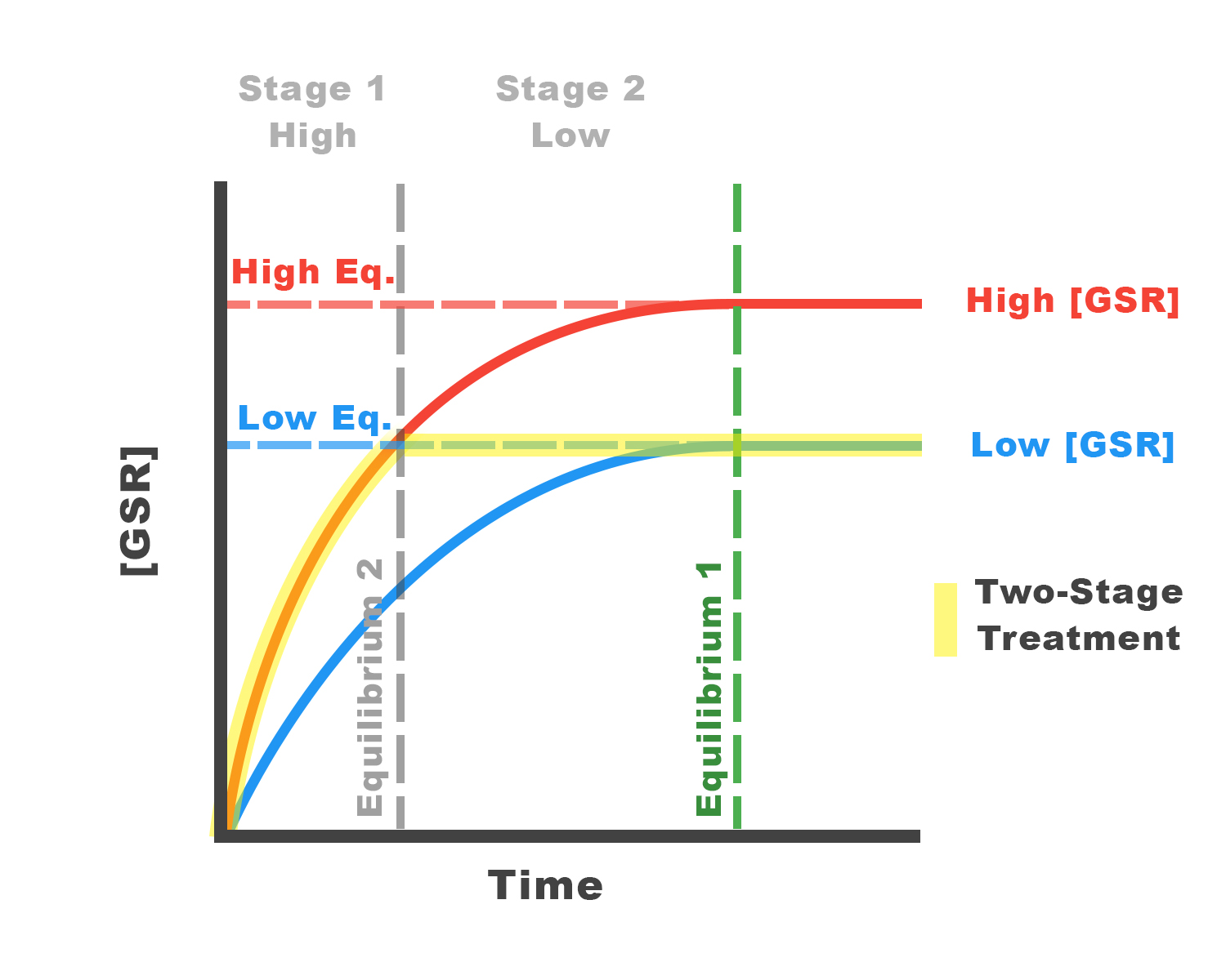
A Two Stage Eyedrop Approach
As shown in Table 2, we cannot alter the time to reach equilibrium, or reach full prevention. As supported by literature research, the time to reach equilibrium is a property of the lens that we cannot change (Fraunfelder 2008). However, we propose a two-stage eyedrop approach, of two differing nanoparticle concentrations, to decrease the time needed for full prevention. A full explanation is found in the collapsible.
Generalized Nanoparticles: Customizer
We built a full nanoparticle customizer, which generalizes the model to beyond delivery into the eye, found at the end of the page (Software). We hope that other iGEM teams who are interested in nanoparticle drug delivery can utilize this customizer to help them develop their own prototype.
Conclusion
We find the optimal combination of parameters is daily doses (high frequency) of 200 nm nanoparticles (small), with a concentration of 76.88 uM of GSR in the nanoparticles (concentration).
Introduction
We do not put GSR directly into eyedrops, because the high turnover rate of the aqueous humor results in a lot of GSR being washed away. Instead, we encapsulate GSR into chitosan nanoparticles, which results in a greater amount of GSR delivered to the lens. This model will quantify the amount of GSR delivered to the lens over time, as new eyedrops are periodically applied.
Analysis of Changing Variables
We vary each variable, nanoparticle radius, concentration, and dose frequency, one at a time, while keeping the other two variables constant.
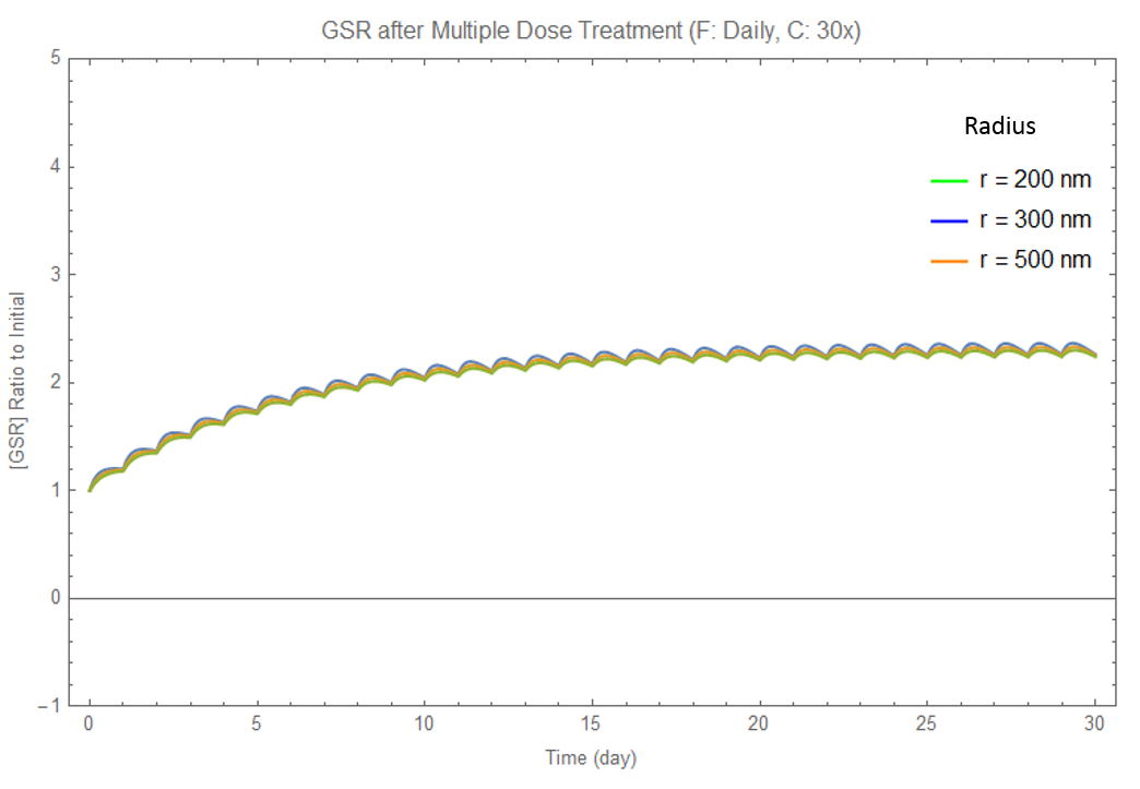
Changing Radius
We find that changing the radius has little impact on the resulting graph, shown in Figure 4.D. Equilibrium is slightly decreased when radius is increased. We will ignore nanoparticle radius. We will use whatever range that is most convienient for manufacturers. For our purposes, we will use r = 200 nm.
Although we disregard nanoparticle radius, this simplification is only true in our desired range of 200 to 400 nm. Extremely small or large nanoparticles will show a difference in release.
Changing Concentration
We find that changing the concentration impacts the equilibrium concentration. There is a direct relationship between GSR concentration inside the nanoparticles, and the equilibrium outside. Higher concentrations also make the graph more unstable, however, shown in a greater amplitude of oscillation in Figure 4.E sample graph is shown above.
Changing Frequency
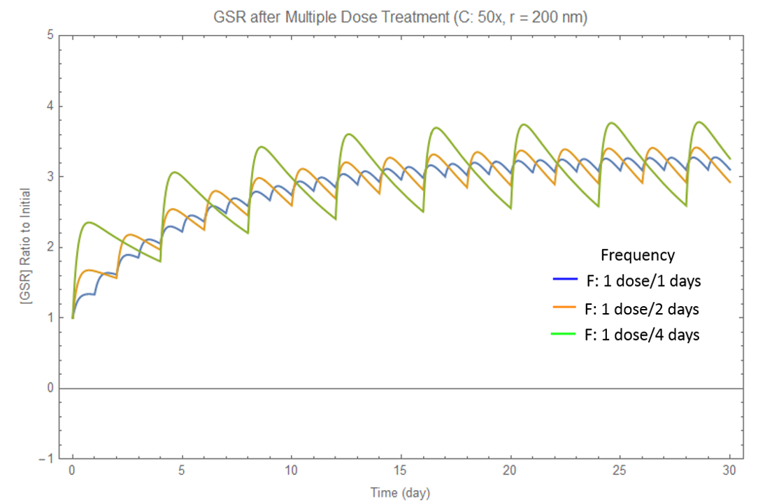
We find that changing the frequency does not impact equilibrium concentration, but does change the stability at equilibrium, as shown in Figure 4.F. The concentration oscillates at a greater amplitude about the equilibrium, which is undesirable, when frequency is too low. Therefore, daily doses are definitely preferred.
We graphed each of the three dependent variables as a function of the three independent variables, and found the quantitative relationship between them. This engineering technique allows us to find an equation for the equilibrium concentration as a function of the three independent variables.
Notice that the time to reach equilibrium (related to the time constant) cannot be altered. See the two eyedrop appraoch to overcome this problem.
Two Stage Eyedrop Approach
Explanation
Problem: We cannot decrease the amount of time until the concentration reaches equilibrium, where full prevention is effective.
Solution: We propose the two stage eyedrop approach. For the first days of treatment, a higher concentration of eyedrop will be used before using a lower concentration. This will speed up the time to reach equilibrium.
In the diagram, we wish to reach the low equilibrium (in blue) as soon as possible. Using the higher concentrated nanoparticles results in the red curve. By applying the higher concentrated nanoparticles in the first days, then switching to the lower concentrated nanoparticles afterwards, we follow the highlighted path. This allows us to reach equilibrium faster.
We need to figure out the concentration of GSR in naoparticles for the blue and red curves. The blue curve (eyedrop 2) requires the original results of our model (outside collapsible). The red curve (eyedrop 1) requires some calculations.
Finding the Concentration of Eyedrop 1
We cannot change the shape of the concentration graphs, because we cannot change the amount of time to reach equilibrium. This means we can find a formula for the percent of GSR delivered. At equilibrium, the value is 1. By curve fitting an exponential to the graph, we find our "percent delivered" function.
The concentration depends on the desired amount of time to reach equilibriu, which we will call "time limit". By plugging the time limit into our percent function, we will know the percentage delivered at the time limit. We divide our goal concentration by this percentage, to find the equilibrium concentration of the red curve. Using the results our model, we can find the concentration of GSR in nanoparticles of eyedrop 1.
We built a functional calculator to find the concentrations of both eyedrops. This is an extention of the eyedrop provided at the bottom of the Model page.
Prevention
Time Limit (Days)
We guarentee that by applying this prevention eyedrop daily, your LOCS score will remain below your threshold for 50 years.
| Variable | Eyedrop 1 | Eyedrop 2 |
|---|---|---|
| Nanoparticle Conc. | uM | uM |
| Eyedrop Result | mg/mL | mg/mL |
Model 4: Eyedrop Prototype
We have found a nanoparticle design to deliver GSR. We also need to model the function of eyedrops, to determine the concentration of GSR-loaded nanoparticles to put in eyedrops, and analyze how sensitive the resulting system is.
Bioavailability of GSR Delivery
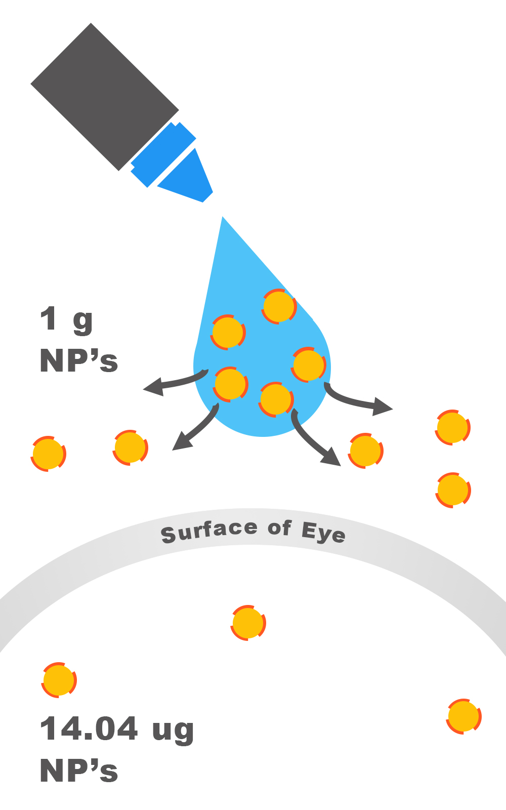
The eye is well protected from foreign material attempting to enter the eye. The corneal epithelium is the most essential barrier against topical drugs in eyedrops, and as a result, much of drugs in eyedrops are lost in tear drainage (Lux 2003).
Bioavailability describes the proportion of the drug that reaches the site of action, regardless of the route of administration. For example, it is estimated that only 1-5% of an active drug with small solutes in an eyedrop penetrates the cornea (Bonate 2005). In the case of nanoparticles, which are much larger than chemical molecules, more is lost (Fraunfelder 2008).
The results show that the bioavailability of nanoparticles is about 1.404 x 10 -3%, which means that for every gram of GSR (or any drug) we place into nanoparticles, approximately 14.04 ug of the drug reach the aqueous humor. The variance is 2.34 ug/g. (Calvo 1996)
Necessary Adjustments in Eyedrops
To ensure that sufficient concentrations of GSR are delivered, we must place an excess of GSR. To determine how much, we simply divide the concentration of GSR in nanoparticles we found in Model 3 by the fraction of GSR that reaches the aqueous humor. This result is programmed in our calculator below.
We conclude that we need 5.48 mM of GSR in nanoparticles in our final eyedrop to maintain 43.5 uM GSR and thus 2.5 LOCS.
Sensitivity Analysis: Revisiting Nanoparticles Model
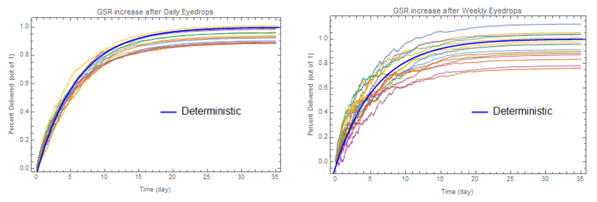
The mechanism for eyedrop delivery is complex, and there are variances in the bioavailability depending on the conditions of the eye (Fraunfelder 2008). The thickness of the cornea, lens, other eye diseases, age, and even time of day may impact the bioavailability of the drug (Gaudana 2010). We use a stochastic model to simulate Model 3 again, but this time, add a degree of variance. The result is shown in Figure 4.10.
The variance is impacted by the frequency of eyedrops. By giving eyedrops more frequently with less amounts given each time, the variance is decreased.
Ideally, we wish to deliver 100% of the GSR concentration of the amount found in Model 2 (43.5 uM). Because of variance, the actual amount maintained in the lens is different, shown in Figure 5. The full details and mathematics of the stochastic model can be found in the collapsible.
Insights into Manufacturing & Clinical Use
Using the details from Models 1-4, we offer the following suggestions for manufacturing our eyedrops, as well as prescribing them to patients.
- Frequent doses of low concentration eyedrops are more stable than occasional doses of high concentration eyedrops. (Model 3)
- Cataract severity is extremely sensitive to the amount of GSR concentration maintained. If this value falls below 43.5 uM even by a little, as shown in Model 2, cataracts may develop. (Model 2)
- When manufacturing, there should be a necessary upward adjustment, because even with daily eyedrops, some simulated trials resulted in less than 90% of GSR delivered. (Model 4)
- Cataract prevention is only fully effective after around 28 days of using the prevention eyedrop. (Model 3) During that time, further cataract damage may take place. The suggested order of treatment should be: start with GSR eyedrops until full prevention is in effect, the use 25HC eyedrops to reverse any existing cataract. Finally, stop 25HC eyedrop use, while continuing GSR eyedrops. (Model 1)
- To speed up the time for full prevention to take place, a two eyedrop approach to quickly deliver sufficient GSR should be used. (Model 4)
Treatment
We use the results from our previous models, and apply them to treatment. The process is almost the exact same as that of Prevention. The only difference is that our treatment protein, CH25H, reverses cataract damage (Griffiths 2016). We find the exact concentration of CH25H to reverse a cataract of a given LOCS score. The delivery models are unchanged, with the exception that the concentration of protein delivery will be different.
We use the results of Model 1 to calculate the LOCS equivalent crystallin damage we need to reverse (“negative crystallin damage”). Then we use experimental results to calculate the concentration of CH25H needed to reverse the cataract. We do not use Model 3, as this is a one-time treatment. After applying the results of Model 4, we can find the final concentration needed in CH25H eyedrops.
We propose eyedrops with 0.8 mg/mL CH25H. The number of drops needed for treatment depends on a patient's current LOCS score, and is calculated in the software tool below.
CALCULATOR
Prevention
LOCS Score Threshold:We guarentee that by applying this prevention eyedrop daily, your LOCS score will remain below your threshold for 50 years.
Prevention Results
| Variable | Value | Source |
|---|---|---|
| Allowable LOCS | ||
| Crystallin Damage | c.d. | Model 1 |
| GSR Maintained | uM | Model 2 |
| Nanoparticle Conc. | uM | Model 3 |
| Eyedrop Conc. | mM | Model 4 |
| Eyedrop Result | mg/mL |
Treatment
Your current LOCS Score:By applying the following treatment, leaving an hour before each dose of eyedrops, we guarentee that it will lower your LOCS score to essentially 0.
Treatment Results
| Variable | Value | Source |
|---|---|---|
| Allowable LOCS | ||
| Crystallin Damage | c.d. | Model 2 |
| Absorbance | a.u. | Model 1 |
| CH25H | uM | Model 5 |
| Eyedrop Conc. | uM | Model 4 |
| Eyedrop Result | mg/mL | Model 4 |
| # of Eyedrops | drops | (of 0.8 mg/mL eyedrop) |
Software
We built a nanoparticle customizer, which allows you to track the concentration and rates of drug delivery to any part of the body using nanoparticles. You can customize your own design of nanoparticles, and analyze its function inside the body.
This computational software can be used by future iGEM teams who are interested in using nanoparticles to efficiently deliver their synthesized proteins. The calculational tool is programmed on a Google Spreadsheet. Click the button below to visit the spreadsheet. Please make a copy of the spreadsheet to freely use it.
Conclusion
The models allowed us to extrapolate short-term experimental data to the long-term, to over 50 years, the duration for cataracts to form. In Models 1-2, with the Cataract Lens Experiments on our synthesized protein GSR (and CH25H), we found the amount of synthesized protein needed in the lens over 50 years. In Models 3-4, with the experimental results of a single dose of nanoparticle release, we simulate multiple doses to see the overall change in GSR concentration in the lens over 50 years. We calculate the exact concentrations of our eyedrop prototype, to prevent a LOCS 2.5 cataract from developing so surgery is not needed. With our predictions and simulations of cataract treatment, we offered insights into how the product should be manufactured and used in clinics. We also programmed a nanoparticle customizer to allow the results of these models to be generalized to all drug delivery iGEM projects.Citation
Adimora, N.J., Jones, D.P., & Kemp, M.L. (2010). A model of redox kinetics implicates the thiol proteome in cellular hydrogen peroxide responses. Antioxidants & Redox Signaling, 13(6), 731-43
Ault, A. (1974). An introduction to enzyme kinetics. Journal of Chemical Education,51(6), 381, DOI: 10.1021/ed051p381
Bonate, P.L., & Howard, D.R. (2005) Pharmacokinetics in Drug Development Volume 2: Regulatory and Development Paradigms. American Association of Pharmaceutical Scientists
CALVO, P., ALONSO, M. J., VILA‐JATO, J. L., & ROBINSON, J. R. (1996). Improved ocular bioavailability of indomethacin by novel ocular drug carriers. Journal of Pharmacy and Pharmacology, 48(11), 1147-1152.
Chylack, L.T., Wolfe, J.K., Singer, D, M., Leske, C., Bullimore, M, A., Bailey, I.L., Friend, J., McCarthy, D., & Wu, S. (1993). The Lens Opacities Classification System III. The Longitudinal Study of Cataract Study Group. American Medical Association. 111(6), 831-36.
Cui, X. L., & Lou, M. F. (1993). The effect and recovery of long-term H 2 O 2 exposure on lens morphology and biochemistry. Experimental eye research, 57(2), 157-167.
Dominguez-Vincent, A., Birkeldh, U., Carl-Gustaf, L., Nilson, M., Brautaset, R., & Al-Ghoul. K.J. (2016).Objective Assessment of Nuclear and Cortical Cataracts through Scheimpflug Images: Agreement with the LOCS III Scale. PLoS One.11(2), doi: 10.1371/journal.pone.0149249
Fraunfelder, F.T., Fraunfelder F.W., & Chambers, W.A.(2008) Clinical Ocular Toxicology: Drug-Induced Ocular Side Effects. Saunders
Gaudana, R., Ananthula, H.K., Parenky, A., Mitra, A.K. (2010). Ocular Drug Delivery. AAPS Journals, 12(3), 348-360 doi: 10.1208/s12248-010-9183-3
Griffiths, W.J., Khalik, J.A., Crick, P.J., Yutuc, E., & Wang, Y. (2016). New methods for analysis of oxysterols and related compounds by LC–MS. Journal of Steroid Biochemistry and Molecular Biology, 162, 4-26, http://dx.doi.ordg/10.1016/j.jsbmb.2015.11.017
Jones, D.P. (2008). Radical-free biology of oxidative stress. American Journal of Physiology. Cell Physiology, 295(4), 849-68
Lux, A., Maier, S., Dinslage, S., Suverkrup, R., & Diestelhorst, M.(2003). A comparative bioavailability study of three conventional eye drops versus a single lyophilisate. British Journal of Ophthalmology, 87(4), 436-440.
Martinovich, G.G., Cherenkevich, & S.N., Sauer. (2005). Intracellular redox state: towards quantitative description. European Biophysics Journal, 34(7), 937-42
Ng, C.F., Schafer, F.Q., Buettner, G.R., & Rodger, V.G.(2007).The rate of cellular hydrogen peroxide removal shows dependency on GSH: mathematical insight into in vivo H2O2 and GPx concentrations. Free Radical Research, 41(11), 1201-11
Norlin, M., Andersson, U., Bjorkhem, I., & Wikvall, Kjell. (2000). Oxysterol 7α-Hydroxylase Activity by Cholesterol 7α-Hydroxylase (CYP7A)*. The American Society for Biochemistry and Molecular Biology, J. Biol. Chem. 34046-34053. doi:10.1074/jbc.M002663200
Salvador, A., Savageau, M.A. (2005). Evolution of enzymes in a series is driven by dissimilar functional demands. National Academy of Sciences of the USA, 103(7), 2226-2231.
Saravanakumar, S., Eswari, A., & Rajendran, L. (2015). Mathematical analysis of immobilized enzyme with reaction-generated pH change on the kinetics using Asymptotic methods.International Journal of Advanced Multidisciplinary Research, 2(8), 98-119
Spector, A., Wang, G.M., Wang, R.R., Garner, W.H., & Moll, H. (1993). The prevention of cataract caused by oxidative stress in cultured rat lenses. I. H2O2 and photochemically induced cataract.Current Eye Research, 12(2), 163-79
Pi, N. A., Yu, Y., Mougous, J. D., & Leary, J. A. (2004). Observation of a hybrid random ping‐pong mechanism of catalysis for NodST: A mass spectrometry approach. Protein science, 13(4), 903-912.
Tajmir-Riahi, H.A., Nafisi, Sh., Sanyakamdhorn, S., Agudelo, D., & Chanphai, P. (2014). Applications of chitosan nanoparticles in drug delivery. Methods in Molecular Biology, 165-84, doi: 10.1007/978-1-4939-0363-4_11
Torchilin, V.P.(2006). Nanoparticles as Drug Carriers. Imperial College Press
Wang, J.J., Zeng, Z.W., Xiao, R.Z., Xie, T., Zhou, G.L., Zhan, X.R., & Wang, S.L. (2011). Recent advances of chitosan nanoparticles as drug carriers. Int J Nanomedicine, 6, 765-774 doi: 10.2147/IJN.S17296
Wong, M.M., Shukla, A.N., & Munir, W.M.(2012). Correlation of corneal thickness and volume with intraoperative phacoemulsification parameters using Scheimpflug imaging and optical coherence tomography. Journal of Cataract & Refractive Surgery, 40(12), 2067-75 doi: 10.1089/ars.2009.2968.

×
Zoom out to see animation.
Your screen resolution is too low unless you zoom out