Difference between revisions of "Team:Pretoria UP/Model"
| (11 intermediate revisions by 2 users not shown) | |||
| Line 18: | Line 18: | ||
<div class="col-md-12"> | <div class="col-md-12"> | ||
| − | <p>A simulation model | + | <p>A simulation model of a PBEC (photo-bioelectrochemical cell) was constructed using AnyLogic. It is to be used for illustrational purposes. |
| − | <br><br>AnyLogic is a simulation | + | <br><br>AnyLogic is a simulation modelling tool that supports multiple simulation methods such as system dynamics, discrete event and agent based modelling. AnyLogic consists of a graphical modelling language working with Java code extensions. |
</p> | </p> | ||
| − | <br> | + | <br> |
| − | <p>Click on the link below to run the simulation model in your browser (Note: Java is required) </p> | + | <p>Click on the link below to run the simulation model in your browser (Note: Java is required) </p> |
| − | <div><table cellpadding="0" cellspacing="0" border="0"><tr><td colspan="2"><a href="http://www.runthemodel.com/models/3101/" target="_blank"><img border="0" alt="Simulation model WattsAptamer: Photo-bioelectrochemical cell created with AnyLogic - simulation software / Synthetic Biology" src="http://www.runthemodel.com/upload/resize_cache/iblock/1da/320_220_1/1da4ed192b4ea32798e214f1957f8bff.png"></a></td></tr><tr><td style="padding-right:10px; padding-top: 2px;" valign="top"><a target="_blank" href="http://www.runthemodel.com/models/run.php?id=3101"><img alt="Run the model" src="http://www.runthemodel.com/img/runthemodel_button.png" border="0"></a></td><td align="right"> | + | <div align="center"> |
| − | <p> If your browser doesn't support Java, see the illustration of the model in action below:</p> | + | <table cellpadding="0" cellspacing="0" border="0"> |
| − | <img style="width:50%" src="https://static.igem.org/mediawiki/2016/e/eb/T--Pretoria_UP--Newmodel.gif"> | + | <tr> |
| − | <br> | + | <td colspan="2"> |
| + | <a href="http://www.runthemodel.com/models/3101/" target="_blank"> | ||
| + | <img border="0" alt="Simulation model WattsAptamer: Photo-bioelectrochemical cell created with AnyLogic - simulation software / Synthetic Biology" src="http://www.runthemodel.com/upload/resize_cache/iblock/1da/320_220_1/1da4ed192b4ea32798e214f1957f8bff.png"></a></td></tr><tr><td style="padding-right:10px; padding-top: 2px;" valign="top"><a target="_blank" href="http://www.runthemodel.com/models/run.php?id=3101"><img alt="Run the model" src="http://www.runthemodel.com/img/runthemodel_button.png" border="0"> | ||
| + | </a> | ||
| + | </td> | ||
| + | <td align="right"> | ||
| + | <a href="http://anylogic.com" target="_blank"> | ||
| + | Developed with | ||
| + | <br>simulation software AnyLogic | ||
| + | </a> | ||
| + | </td> | ||
| + | </tr> | ||
| + | </table> | ||
| + | </div> | ||
| + | |||
| + | <br><p> If your browser doesn't support Java, see the illustration of the model in action below:</p> | ||
| + | <p style="text-align:center"> | ||
| + | <img style="width:50%" src="https://static.igem.org/mediawiki/2016/e/eb/T--Pretoria_UP--Newmodel.gif"> | ||
| + | </p> | ||
| + | <br><br> | ||
<p><b>"Black box" strategy</b> | <p><b>"Black box" strategy</b> | ||
| Line 33: | Line 52: | ||
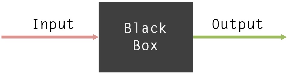
<p>In order to reduce the complexity of the simulation model, a “black box” strategy was followed. A “black box model” requires specific information as input where after the system utilizes pre-programmed logic to return output to the user. Many “black box models” can be used which uses each other’s output (Investopedia, 2016). Making use of a “black box model” ensured that functional areas relevant to the proposed model were isolated without neglecting variability, as a result of the influence of other parameters. | <p>In order to reduce the complexity of the simulation model, a “black box” strategy was followed. A “black box model” requires specific information as input where after the system utilizes pre-programmed logic to return output to the user. Many “black box models” can be used which uses each other’s output (Investopedia, 2016). Making use of a “black box model” ensured that functional areas relevant to the proposed model were isolated without neglecting variability, as a result of the influence of other parameters. | ||
</p> | </p> | ||
| − | <img style="max-width:50%" src="https://static.igem.org/mediawiki/2016/8/82/T--Pretoria_UP--Simulation_Model_1.jpg"> | + | <div align="center"> |
| + | <img style="max-width:50%" src="https://static.igem.org/mediawiki/2016/8/82/T--Pretoria_UP--Simulation_Model_1.jpg"> | ||
| + | <br> | ||
| + | <br> | ||
| + | <p style="font-size:14px !important;text-align:center;">Figure 1: A simple “black box” model | ||
| + | </p> | ||
| + | </div> | ||
<br> | <br> | ||
| − | |||
| − | |||
| − | |||
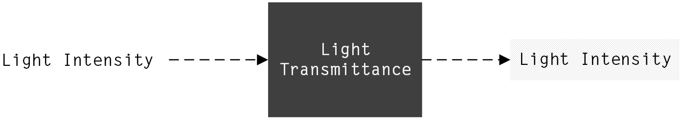
<p>The first “black box” to be addressed relates to the influence of the material type used for the casing of the battery. Perspex and glass were considered as possibilities. Absorption properties of material influence transmitted light. This will in return affect the light reaching the attached photosystems. Perspex of 4.5 mm thick has a solar light transmittance of 37% and visible light transmittance of 33%. Glass has a solar transmittance of 90% and visible light transmittance of 91% (Altuglas International, 2016). | <p>The first “black box” to be addressed relates to the influence of the material type used for the casing of the battery. Perspex and glass were considered as possibilities. Absorption properties of material influence transmitted light. This will in return affect the light reaching the attached photosystems. Perspex of 4.5 mm thick has a solar light transmittance of 37% and visible light transmittance of 33%. Glass has a solar transmittance of 90% and visible light transmittance of 91% (Altuglas International, 2016). | ||
<br><br>A changed light intensity | <br><br>A changed light intensity | ||
<math>(μ mole photons.m<sup>−2</sup>.s<sup>−1</sup>) | <math>(μ mole photons.m<sup>−2</sup>.s<sup>−1</sup>) | ||
</math> | </math> | ||
| − | is obtained as an output as seen in Figure | + | is obtained as an output as seen in Figure 2 below. |
</p> | </p> | ||
| − | <img style="max-width:75%" src="https://static.igem.org/mediawiki/2016/2/20/T--Pretoria_UP--Simulation_Model_2.jpg"> | + | <div align="center"> |
| − | + | <img style="max-width:75%" src="https://static.igem.org/mediawiki/2016/2/20/T--Pretoria_UP--Simulation_Model_2.jpg"> | |
| − | + | <br> | |
| + | <p style="font-size:14px !important;text-align:center;">Figure 2: The first “black box” | ||
| + | </div> | ||
</p> | </p> | ||
<br> | <br> | ||
| Line 52: | Line 76: | ||
</p> | </p> | ||
<p>The second “black box” in the model represents the process of photosynthesis occurring in photosystems within the attached thylakoid membranes. | <p>The second “black box” in the model represents the process of photosynthesis occurring in photosystems within the attached thylakoid membranes. | ||
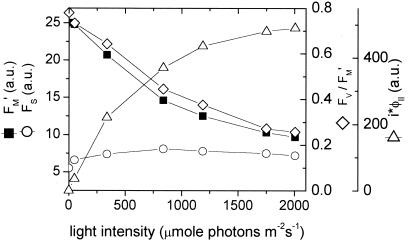
| − | <br><br>Photosynthetic electron transfer’s relative proton to electron stoichiometries (H+/e- ratios) was obtained from living tobacco plant leaves under steady-state illumination. Electron transfer fluxes as well as turnover rates of linear electron transfer through the cytochrome (cyt) b6f complex were estimated (Colette A. Sacksteder, 2000). In Figure | + | <br><br>Photosynthetic electron transfer’s relative proton to electron stoichiometries (H+/e- ratios) was obtained from living tobacco plant leaves under steady-state illumination. Electron transfer fluxes as well as turnover rates of linear electron transfer through the cytochrome (cyt) b6f complex were estimated (Colette A. Sacksteder, 2000). In Figure 3, fluorescence yields and electron flux of photosystem II is plotted. Yields from fluorescence during saturation pulses, |
<math><i>F'</i><sub>M</sub> | <math><i>F'</i><sub>M</sub> | ||
</math> | </math> | ||
| Line 67: | Line 91: | ||
</p> | </p> | ||
<br> | <br> | ||
| − | <img style="max-width:75%" src="https://static.igem.org/mediawiki/2016/1/17/T--Pretoria_UP--Simulation_Model_3.jpg"> | + | <div align="center"> |
| − | + | <img style="max-width:75%" src="https://static.igem.org/mediawiki/2016/1/17/T--Pretoria_UP--Simulation_Model_3.jpg"> | |
| − | + | <br> | |
| − | + | <br> | |
| − | + | <p style="font-size:14px !important;text-align:center;">Figure 3: Photosystem II electron flux and various fluorescence yields as a function of light intensity | |
| + | </p> | ||
| + | |||
| + | </div> | ||
<br> | <br> | ||
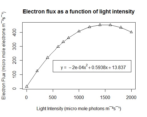
<p>The estimate of electron flux | <p>The estimate of electron flux | ||
<math>(<i>i</i>⋅Φ<sub>II</sub>) | <math>(<i>i</i>⋅Φ<sub>II</sub>) | ||
</math> | </math> | ||
| − | (open diamonds) is of importance in describing what happens in the second “black box” of this simulation model. A line of best fit was retrieved from the information in Figure | + | (open diamonds) is of importance in describing what happens in the second “black box” of this simulation model. A line of best fit was retrieved from the information in Figure 3 and transformed to a polynomial function plotted in Figure 3, described by the following equation: |
</p> | </p> | ||
<p style="text-align:center;"> | <p style="text-align:center;"> | ||
| Line 83: | Line 110: | ||
</math> | </math> | ||
</p> | </p> | ||
| − | <img style="max-width:75%" src="https://static.igem.org/mediawiki/2016/b/b5/T--Pretoria_UP--Simulation_Model_4.jpg"> | + | <div align="center"> |
| − | + | <img style="max-width:75%" src="https://static.igem.org/mediawiki/2016/b/b5/T--Pretoria_UP--Simulation_Model_4.jpg"> | |
| − | + | <br> | |
| − | + | <p style="font-size:14px !important;text-align:center;">Figure 4: Electron flux of photosystem II as a function of light intensity | |
| + | </p> | ||
| + | </div> | ||
<br> | <br> | ||
<p>The above figure describes the electron flux obtained from a single photosystem II. There is a single photosystem II inside each | <p>The above figure describes the electron flux obtained from a single photosystem II. There is a single photosystem II inside each | ||
| Line 93: | Line 122: | ||
thick thylakoid (Kirschner Lab, 2001). | thick thylakoid (Kirschner Lab, 2001). | ||
<br><br>This was used to calculate the quantity of photosystems II possibly located on the surface area of the graphene electrode. | <br><br>This was used to calculate the quantity of photosystems II possibly located on the surface area of the graphene electrode. | ||
| − | <br><br><img style="max-width:75%" src="https://static.igem.org/mediawiki/2016/b/b3/T--Pretoria_UP--Simulation_Model_5.jpg"> | + | |
| − | + | <div align="center"> | |
| − | + | <br><br><img style="max-width:75%" src="https://static.igem.org/mediawiki/2016/b/b3/T--Pretoria_UP--Simulation_Model_5.jpg"> | |
| − | + | <br> | |
| − | <br>As seen in the above Figure | + | <p style="font-size:14px !important;text-align:center;">Figure 5: The second "black box" |
| + | </p> | ||
| + | </div> | ||
| + | <br>As seen in the above Figure 5, light intensity | ||
<math>(μ mole photons m<sup>−2</sup>s<sup>−1</sup>) | <math>(μ mole photons m<sup>−2</sup>s<sup>−1</sup>) | ||
</math> | </math> | ||
| Line 179: | Line 211: | ||
</p> | </p> | ||
<br> | <br> | ||
| − | <img width="75%" style="max-width:100%" src="https://static.igem.org/mediawiki/2016/1/11/T--Pretoria_UP--Simulation_Model_6.jpg"> | + | <div align="center"> |
| + | <img width="75%" style="max-width:100%" src="https://static.igem.org/mediawiki/2016/1/11/T--Pretoria_UP--Simulation_Model_6.jpg"> | ||
| + | <br> | ||
| + | <p style="font-size:14px !important;text-align:center;">Figure 6: The third "black box" | ||
| + | </p> | ||
| + | </div> | ||
<br> | <br> | ||
| − | + | <p>In the above Figure 6, electron flux | |
| − | + | ||
| − | + | ||
| − | <p>In the above Figure | + | |
<math>(μ mole electrons.m<sup>−2</sup>.s<sup>−1</sup>) | <math>(μ mole electrons.m<sup>−2</sup>.s<sup>−1</sup>) | ||
</math> | </math> | ||
| Line 191: | Line 225: | ||
<p><b>The Overall Model Logic</b> | <p><b>The Overall Model Logic</b> | ||
</p> | </p> | ||
| − | <p>Combining all of the “black boxes” results in the model logic as illustrated in Figure | + | <p>Combining all of the “black boxes” results in the model logic as illustrated in Figure 7. Changeable parameters include: light intensity |
<math>(μ mole photons.m<sup>−2</sup>.s<sup>−1</sup>), | <math>(μ mole photons.m<sup>−2</sup>.s<sup>−1</sup>), | ||
</math> | </math> | ||
casing material (Perspex or glass), electrode size and whether or not to select thylakoid attachment by making use of aptamers. The main measurable is current (A). | casing material (Perspex or glass), electrode size and whether or not to select thylakoid attachment by making use of aptamers. The main measurable is current (A). | ||
</p> | </p> | ||
| − | <img style="max-width:75%" src="https://static.igem.org/mediawiki/2016/d/d9/T--Pretoria_UP--Simulation_Model_7.jpg"> | + | <div align="center"> |
| − | + | <img style="max-width:75%" src="https://static.igem.org/mediawiki/2016/d/d9/T--Pretoria_UP--Simulation_Model_7.jpg"> | |
| − | + | <br> | |
| − | + | <p style="font-size:14px !important;text-align:center;">Figure 7: The combination of "black boxes" used in the model | |
| + | </p> | ||
| + | </div> | ||
<br> | <br> | ||
<p><b>User Interface and Animation</b> | <p><b>User Interface and Animation</b> | ||
| Line 207: | Line 243: | ||
<p><b>Model Results</b> | <p><b>Model Results</b> | ||
</p> | </p> | ||
| + | |||
| + | <p>In order to illustrate the results of the simulation model, 3D graphs were compiled of the output obtained from each “black box”. Following is a graph that displays the light intensity obtained after using Perspex and glass of both 0.2 and 0.5 mm thick at various input light intensities. As illustrated, the highest yield is obtained by using 0.2 mm thick glass at a light intensity of <math>1840 μ mole photons.m<sup>−2</sup>.s<sup>−1</sup>; | ||
| + | </math></p> | ||
| + | <br> | ||
| + | <br> | ||
| + | <div align="center"> | ||
| + | <img width="75%" style="max-width:100%" src="https://static.igem.org/mediawiki/2016/5/5f/T--Pretoria_UP--ResultsGraph1.png"> | ||
| + | <br> | ||
| + | <br> | ||
| + | <p style="font-size:14px !important;text-align:center;">Figure 8: Model results of adapted light intensity related to different material types | ||
| + | </p> | ||
| + | </div> | ||
| + | <br> | ||
| + | <p>The process of photosynthesis occurring in the thylakoid membranes is represented by the second “black box”. Following is a graph of the obtained electron flux as a result of both the electrode size (surface area) and light intensity. The highest yield is observed in the region using an electrode surface area of <math>6.9 cm<sup>2</sup></math> and light intensity of <math>1840 μ mole photons.m<sup>−2</sup>.s<sup>−1</sup>; | ||
| + | </math>.</p> | ||
| + | <br> | ||
| + | <br> | ||
| + | <div align="center"> | ||
| + | <img width="75%" style="max-width:100%" src="https://static.igem.org/mediawiki/2016/3/3d/T--Pretoria_UP--ResultsGraph2.png"> | ||
| + | <br> | ||
| + | <br> | ||
| + | <p style="font-size:14px !important;text-align:center;">Figure 9: Model results of electron flux as a result of electrode size and light intensity | ||
| + | </p> | ||
| + | </div> | ||
| + | <br> | ||
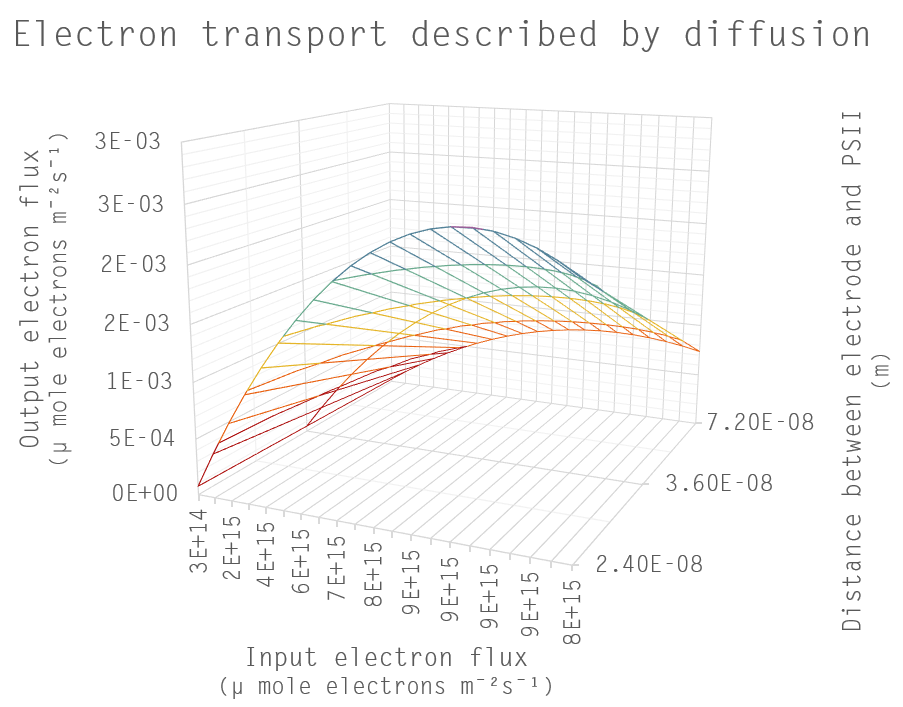
| + | <p>The third “black box” represents electron transport from the thylakoid membranes to the graphene electrode via diffusion. Following is a graph of the adjusted electron flux after electron diffusion occurred. The highest output electron flux is obtained by using an input electron flux of <math>8 × 10<sup>15</sup></math> μ mole electrons.m<sup>−2</sup>.s<sup>−1</sup>; with the smallest possible distance between the electrode and the thylakoid membranes. This shortest distance is obtained by making use of aptamers of length <math>2.4 × 10<sup>−8</sup> m that binds explicitly to the graphene electrode and thylakoid membranes. </p> | ||
| + | <br> | ||
| + | <br> | ||
| + | <div align="center"> | ||
| + | <img width="75%" style="max-width:100%" src="https://static.igem.org/mediawiki/2016/c/c3/T--Pretoria_UP--ResultsGraph3.png"> | ||
| + | <br> | ||
| + | <br> | ||
| + | <p style="font-size:14px !important;text-align:center;">Figure 10: Model results of adjusted electron flux after diffusion occurred | ||
| + | </p> | ||
| + | </div> | ||
| + | <br> | ||
| + | |||
<p>After multiple runs, the highest yield resulting in a current of | <p>After multiple runs, the highest yield resulting in a current of | ||
<math>5.342 × 10<sup>−21</sup>A | <math>5.342 × 10<sup>−21</sup>A | ||
Latest revision as of 20:10, 19 October 2016
Simulation Model A simulation model of a PBEC (photo-bioelectrochemical cell) was constructed using AnyLogic. It is to be used for illustrational purposes.
Click on the link below to run the simulation model in your browser (Note: Java is required) If your browser doesn't support Java, see the illustration of the model in action below:
"Black box" strategy
In order to reduce the complexity of the simulation model, a “black box” strategy was followed. A “black box model” requires specific information as input where after the system utilizes pre-programmed logic to return output to the user. Many “black box models” can be used which uses each other’s output (Investopedia, 2016). Making use of a “black box model” ensured that functional areas relevant to the proposed model were isolated without neglecting variability, as a result of the influence of other parameters.
Figure 1: A simple “black box” model
The first “black box” to be addressed relates to the influence of the material type used for the casing of the battery. Perspex and glass were considered as possibilities. Absorption properties of material influence transmitted light. This will in return affect the light reaching the attached photosystems. Perspex of 4.5 mm thick has a solar light transmittance of 37% and visible light transmittance of 33%. Glass has a solar transmittance of 90% and visible light transmittance of 91% (Altuglas International, 2016).
Figure 2: The first “black box”
The second "black box"
The second “black box” in the model represents the process of photosynthesis occurring in photosystems within the attached thylakoid membranes.
Figure 3: Photosystem II electron flux and various fluorescence yields as a function of light intensity
The estimate of electron flux
(open diamonds) is of importance in describing what happens in the second “black box” of this simulation model. A line of best fit was retrieved from the information in Figure 3 and transformed to a polynomial function plotted in Figure 3, described by the following equation:
Figure 4: Electron flux of photosystem II as a function of light intensity
The above figure describes the electron flux obtained from a single photosystem II. There is a single photosystem II inside each
thick thylakoid (Kirschner Lab, 2001).
Figure 5: The second "black box"
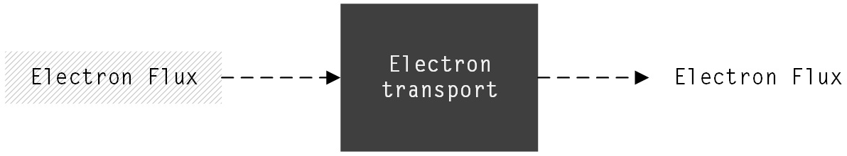
The third "black box"
Fick’s diffusion laws are used to describe the movement of electrons from the photosystems to the graphene electrode. Fick’s first law is given as:
Where
Equation [2] can be rearranged into Equation [3]:
Where
The concentration of electrons at point 1 is the changing electron flux produced by the thylakoid membranes and obtained from the second “black box”. It is assumed that the electron concentration at point 2, which is the surface area of the graphene electrode, is infinitely small. The exposed surface area (A) of the graphene electrode is where the thylakoid membranes are attached. The distance (x) resembles the space between the thylakoid membrane and the surface area of the graphene. Using aptamers, this distance amounts to
(Barendse, 2016). Without the use of aptamers an 50% increase in distance is assumed.
Where
Boltzmann’s constant of
is used. An absolute temperature of 273.16 K is assumed as the battery will be operating at room temperature. The electric mobility in water of
is used. The diffusion coefficient
is calculated as
Figure 6: The third "black box"
In the above Figure 6, electron flux
is used as input for the second black box, where after equation [3] and [4] describe the diffusion of electrons from the thylakoid membranes to the graphene electrode. An output of a number of electrons per second is obtained.
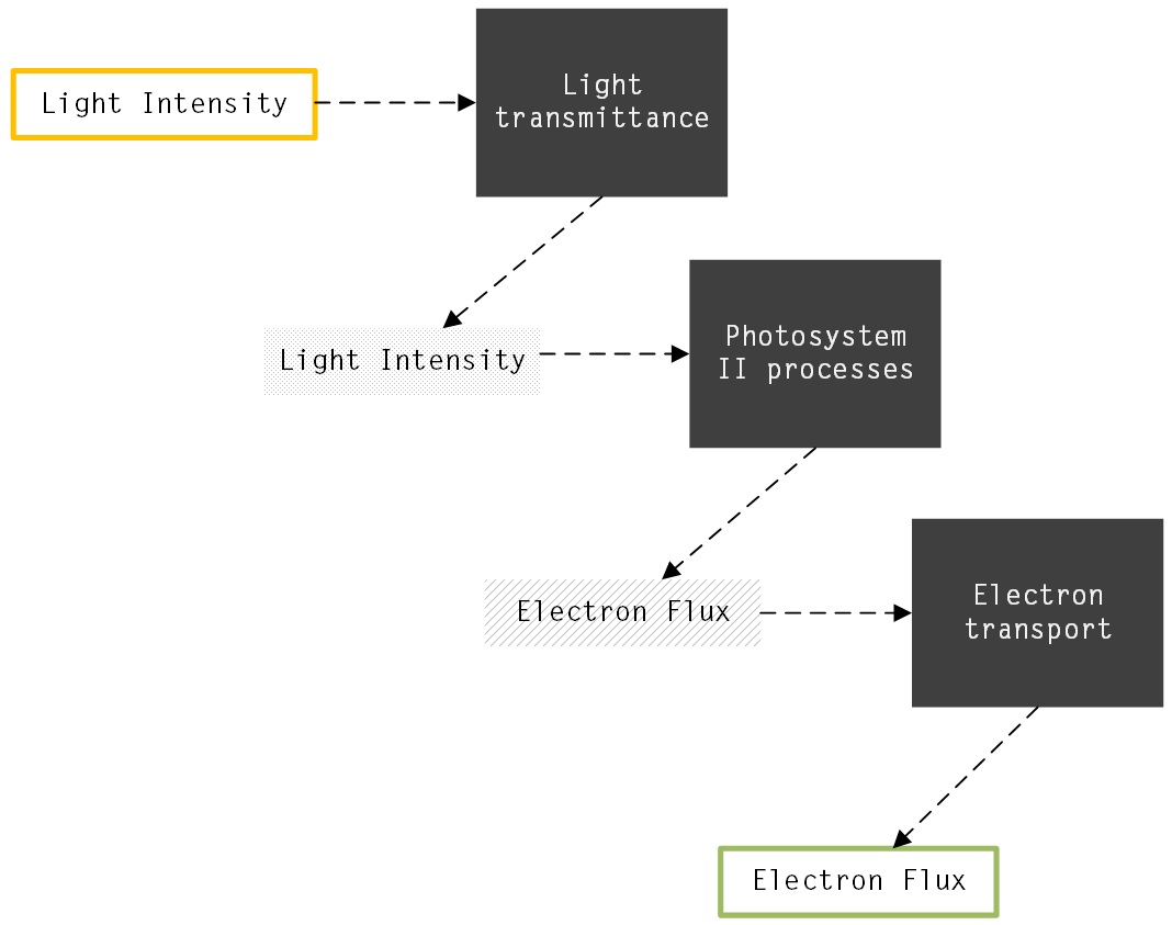
The Overall Model Logic
Combining all of the “black boxes” results in the model logic as illustrated in Figure 7. Changeable parameters include: light intensity
casing material (Perspex or glass), electrode size and whether or not to select thylakoid attachment by making use of aptamers. The main measurable is current (A).
Figure 7: The combination of "black boxes" used in the model
User Interface and Animation
Buttons and sliders are added to allow the user to change specific parameters. Graphs of both the current (A) measured and the influence of light intensity on the electron flux produced are drawn dynamically. A 3D illustration of the PBEC is also presented which is animated as the user changes parameters.
Model Results
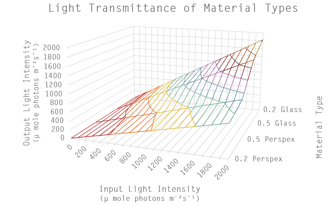
In order to illustrate the results of the simulation model, 3D graphs were compiled of the output obtained from each “black box”. Following is a graph that displays the light intensity obtained after using Perspex and glass of both 0.2 and 0.5 mm thick at various input light intensities. As illustrated, the highest yield is obtained by using 0.2 mm thick glass at a light intensity of Figure 8: Model results of adapted light intensity related to different material types
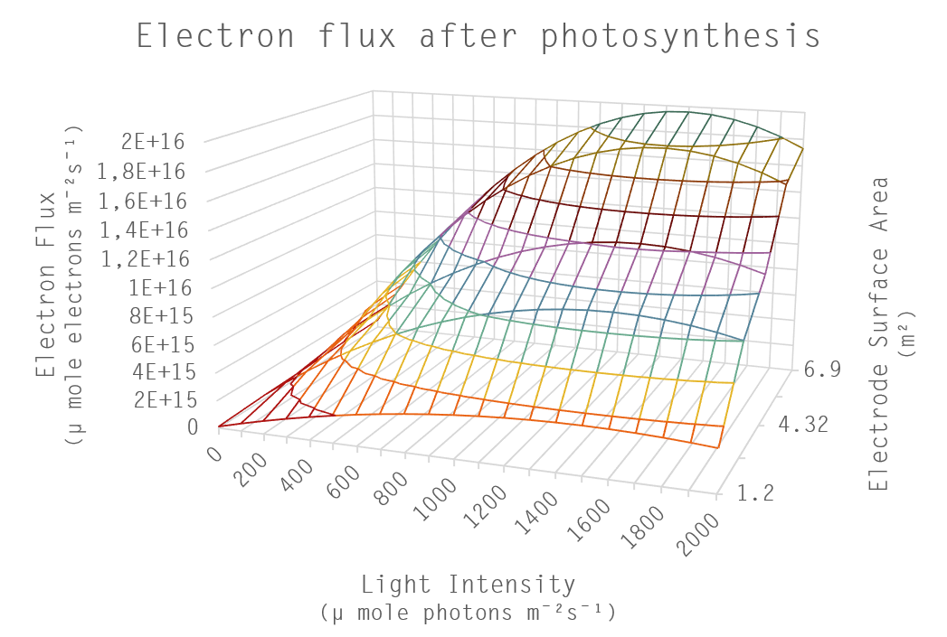
The process of photosynthesis occurring in the thylakoid membranes is represented by the second “black box”. Following is a graph of the obtained electron flux as a result of both the electrode size (surface area) and light intensity. The highest yield is observed in the region using an electrode surface area of and light intensity of . Figure 9: Model results of electron flux as a result of electrode size and light intensity
The third “black box” represents electron transport from the thylakoid membranes to the graphene electrode via diffusion. Following is a graph of the adjusted electron flux after electron diffusion occurred. The highest output electron flux is obtained by using an input electron flux of μ mole electrons.m−2.s−1; with the smallest possible distance between the electrode and the thylakoid membranes. This shortest distance is obtained by making use of aptamers of length Figure 10: Model results of adjusted electron flux after diffusion occurred
After multiple runs, the highest yield resulting in a current of
was obtained with the following parameter settings: Light intensity of
using glass as casing material; keeping the electrode surface area at
making use of aptamers to attach thylakoids to the electrode.
AnyLogic is a simulation modelling tool that supports multiple simulation methods such as system dynamics, discrete event and agent based modelling. AnyLogic consists of a graphical modelling language working with Java code extensions.
A changed light intensity
is obtained as an output as seen in Figure 2 below.
Photosynthetic electron transfer’s relative proton to electron stoichiometries (H+/e- ratios) was obtained from living tobacco plant leaves under steady-state illumination. Electron transfer fluxes as well as turnover rates of linear electron transfer through the cytochrome (cyt) b6f complex were estimated (Colette A. Sacksteder, 2000). In Figure 3, fluorescence yields and electron flux of photosystem II is plotted. Yields from fluorescence during saturation pulses,
(closed squares) and yields from fluorescence in the steady-state,
>
(open circles), were obtained at varying light intensities. Photosystem II and associated light-harvesting complexes’
quantum yield and an estimate of the electron flux of photosystem II
were calculated, as described in the above mentioned report.
This was used to calculate the quantity of photosystems II possibly located on the surface area of the graphene electrode.
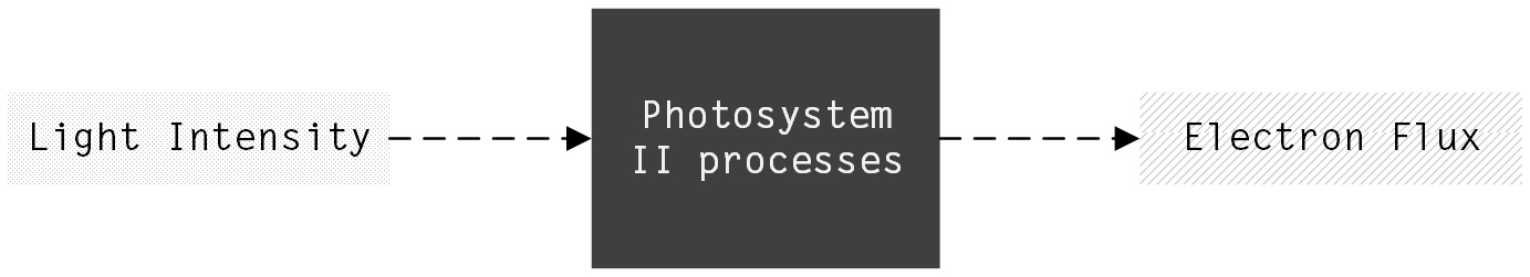
As seen in the above Figure 5, light intensity
is used as input for the first black box, where after equation [1] describes processes happening inside the box and gives an output of electron flux
The diffusion coefficient of electrons in solution is calculated using Einstein’s relation, also known as Einstein–Smoluchowski relation: