1) Established a general idea of how our system works (Metal Aptamer sensor and Leptospirosis detector).
2) Constructed useful reaction schemes to represent how our system works.
3) Derived differential equations from reaction scheme using mathematical laws.
4) Estimated reaction constants by reading through related literature and using acquired information to make reasonable estimations.
5) Implemented differential equations with related reaction constants into MATLAB as functions.
6) Produced graphical representations showing fluctuations in molecule number of each species.
7) Devised potential experiments that could be conducted to characterise/parameterise model more accurately.
Team:Warwick/Model
Summary
Introduction
The Warwick iGEM team decided to use a CRISPR/Cas9 system to build a sensing device for Leptospirosis detection. CRISPR technology is a relatively new, not fully understood technology, so for our project to be successful, it was imperative that we have as detailed an understanding of the way the technology operates as possible. As a result, we spent a lot of time trying to develop a model that accurately represents the behaviour of our system.
How the system works/What parts we decided to model?
For us to be able to model our system, we had to establish what we thought would be happening while our device was in action. Before our system could start sensing Leptospirosis RNA, we had to produce the three plasmids that in turn produced the sensing complex. Once these plasmids had been constructed, the sensing process could begin.
At the start of the sensing process, when our system is in any environment, Plasmid 1 produces the dCas9. Plasmid 1 is also capable of making GFP. Plasmid 2 produces the RNA binding protein with the attached Effector while Plasmid 3 makes the sgRNA. All of these products are released into the surrounding environment in large quantities.
Our sgRNA design incorporates a region that is complementary to dCas9 molecules that we call the dCas9 handle. When the sgRNA is in its original shape, the handle is not accessible to the dCAs9, however, if there is Leptospirosis RNA present in the environment, it will bind to the sgRNA, changing its shape and allowing the dCAs9 to bind to it.
The dCas9/sgRNA complex is guided back to Plasmid 1 by the dCas9 component. When the dCas9/sgRNA complex is bound to Plasmid 1, the dCas9 molecule then acts as a beacon for the RNA binding protein with the attached effector to find the sgRNA and bind to it.
When the previous binding process is complete, the RNA binding protein/effector recruits an RNA polymerase, allowing it to read the gene for GFP production present on Plasmid 1. GFP is produced and is released into the surrounding environment.
When establishing the way that our system operates, we made the following assumptions to make the modelling process easier:
1) Each step of the process happens one step at the time (so two species binding simultaneously does not happen).
2) The RNA being sensed has a strong binding affinity to our sgRNA and will not unbind once bound.
3) The sgRNA will be produced in relative abundance relative to the other species in the environment.
After having established the way we expected our system to perform, we decided that it would be most useful to model the rate of change of concentration for the different molecules that would be present in our system at any given time.
Our ultimate goal was to accurately predict the amount of GFP being produced. This would give us an insight into how sensitive our detection device will be with differing amounts of Leptospirosis RNA present in a system.
Method
In order to start modelling our system, we needed to construct a reaction scheme to apply modelling techniques to. The aim of applying these modelling techniques to our reaction was to derive ordinary differential equations that would dynamically represent the behaviour of our system over a given period of time. We will now explain the process that we went through to refine our reaction scheme, in the hope that future iGEM teams may learn from our mistakes or improve on our model.
Initially, we constructed a reaction scheme that showed step by step what would happen when our system is detecting Leptospirosis, in the case where the Leptospirosis RNA is present. This reaction scheme is shown below:
1) T0→mRNA→ dCas9
2) T0→ mRNA→ RNABP + Eff
3) T0→sgRNA→ sgRNA + Leptospirosis RNA
4) sgRNA + dCas9 + RNABP/Eff ↔ dCas9*
5) dCas9* + Plasmid 1 → Plasmid 1*
6) RNABP/Effector + RNA Polymerase ↔ Active RNA Polymerase
7) Active RNA Polymerase → GFP
ODEs from this reaction scheme: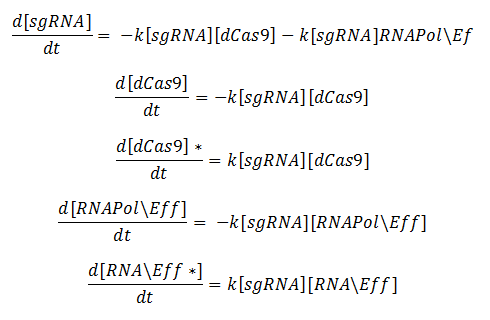
Model for GFP Production: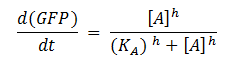
Key: T0 = Starting time, dCas9 = deactivated Cas9, RNABP = RNA Binding Protein, Eff = Effector, GFP = Green fluorescent Protein, KA = Association constant, h = Hill coefficient, A = Active RNA Polymerase
The ODEs were derived by applying the law of mass action to the reaction scheme. To model the production of GFP, we used a Hill activation function. These modelling techniques are explained in more detail later on.
We came to realise that the reaction scheme above is not an accurate representation of what could actually happen in our system. It only showed what would happen with our system in the ideal case, being that everything formed at the right time and in the right order with Leptospirosis RNA present in the system. It was possible for our full activation complex to be formed in different orders.
For example, it was possible for our sgRNA to bind to the plasmid before or after it had bound the RNA binding protein. This is significant because the association/dissociation constants for the different potential formation processes mean that the concentrations of the different species may be slightly different.
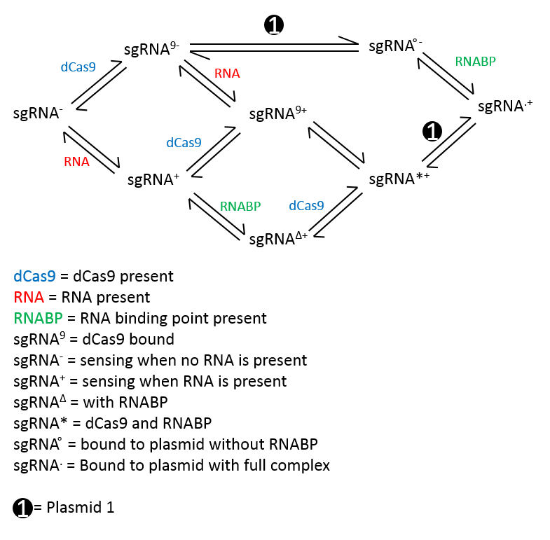
So we then decided to construct another reaction scheme that showed in greater detail what was going on when our system detects Leptospirosis. This reaction scheme assumed that only one process could happen at a time.
General ODEs derived from this reaction scheme: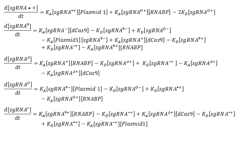
We felt that the second reaction scheme was a lot more accurate with regards to representing our system. Another advantage of using this reaction scheme is that it showed the reversibility in all of the steps. However, it immediately became apparent that this reaction scheme may cause confusion.
Consequently, we decided against using this reaction scheme. In addition to causing confusion, this reaction was flawed because it doesn’t show the production of GFP, but only the production of the complex that produces GFP. Also, due to the nature of the GFP that we were using, we had to take into account degradation of GFP due to the degradation tag and diffusion.
Hence, it was clear that we needed to produce an improved reaction scheme. So we reconstructed our reaction scheme one last time. This process yielded the following result:
1. A → ᵠ
2. ᵠ → gR → ᵠ
3. ᵠ → sR → ᵠ
4. ᵠ → eC→ ᵠ
5. ᵠ → B→ ᵠ
6. gR + sR↔ fR
7. gR + eC ↔ gC
8. fR + eC ↔ fC
9. fC + B ↔ A
10. A → P
11. P → ᵠ
12. P → ᵠ
Key:
A – Full activation complex that will start transcription of GFP (With fR, eC and B, all bound together)
P – Protein output (GFP)
B – RNA Binding Protein
gR – Our designed sgRNA
sR – Leptospirosis RNA
fR – sgRNA bound to Leptospirosis RNA
fC – Complex with fR and eC present
gC – Complex with gR and eC present (Complex formed when guide RNA binds to dCas9 without binding to Leptospirosis disease RNA)
eC – dCas9 molecule
Assumptions:
- Assumed that dCas9 could still bind to sgRNA without the Leptospirosis RNA, to find the likelihood of us obtaining the false positive.
ODEs from this reaction scheme: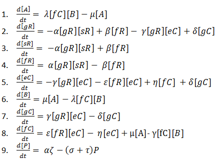
We decided that this reaction scheme would be the one most suitable to base our mathematical modelling on as it manages to accurately represent as many of the steps that our system goes through as simply as possible.
The production of the actual protein (GFP), P, is dependent on many conditions being fulfilled, so using mass action kinetics to derive ODEs to represent this would not be appropriate. To overcome this problem, we decided to use the Shea-Ackers formalism (Equation 9). More information about this method of modelling gene regulation is described below.
ODE Equation Key:
τ = Degradation of GFP due to dilution
σ = Degradation of GFP due to degradation tag.
Once all of our ODEs had been derived, we implemented them as functions on MATLAB. We then inserted the relevant binding constants and generated plots to see how the species prevalent in our system varied.
Results
The Ideal Case
The Warwick iGEM team decided that it would be useful to test the model first by running it using completely idealised parameters. We created this idealised model in order to represent how we would expect our system to work. Fabricating this model also allowed us to have a base to compare the models with more realistic parameters to.
In this idealised model, the reaction constants relevant to each of the equations that modelled the rate of change of molecule number of each of the species, in a single cell, were chosen to give us the most desirable output.
In this case we picked our initial condition so that they were consistent with values that had already been obtained in from other experiments. These values are displayed in the parameters table.
Figures 1, 2 and 3 are illustrations of our model, showing how the different species in our system will fluctuate in molecule number over time. The number of Leptospirosis (sR), sgRNA (gR) an dCas9 (eC) molecules start off with relatively high values, but quickly decline as they all bind together to form the ‘fR’ complex, hence why the number of ‘fR’ molecules start at zero then slowly increases. There is a more delayed decline in the molecule number of the RNA Binding Protein (B) as the ‘fR’ complex needs to be formed first. Once all of the ‘fC’ molecules are formed, then molecules of the full GFP activation complex ‘A’ are formed and in turn GFP production ‘P’ begins.
Realistic Case
After having produced illustrations of the ideal behaviour of our system, we decided to try and parameterise our model using values from the literature, as we were unable to determine them experimentally. The values that we obtained were used to provide the illustrations shown in figures 4, 5 and 6.
These illustrations don’t really match how we expect our system to operate and we feel that this could be down to any of the following reasons:
- The parameters obtained from the literature, although partially relevant, are not accurate parameters when used to model our system, as they may have been obtained in different conditions to those that our system operates in (e.g in vivo as opposed to in vitro)
- Our model does not account for all of the molecule reactions that occur while our system is sensing RNA
For our model to be fully characterised and tested for robustness, further experiments will need to be conducted, in order to determine the appropriate reaction constants.
Shown in the table below are the parameters used to generate the illustrations of the ideal case and realistic case.
Paramter Table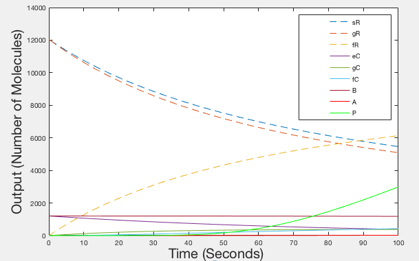
Figure 1: Graph of Ideal behaviour - Timespan 100 seconds
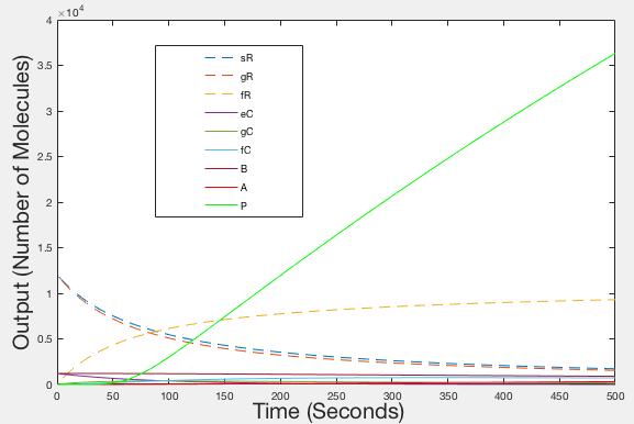
Figure 2: Graph of Ideal behaviour - Timespan 500 seconds
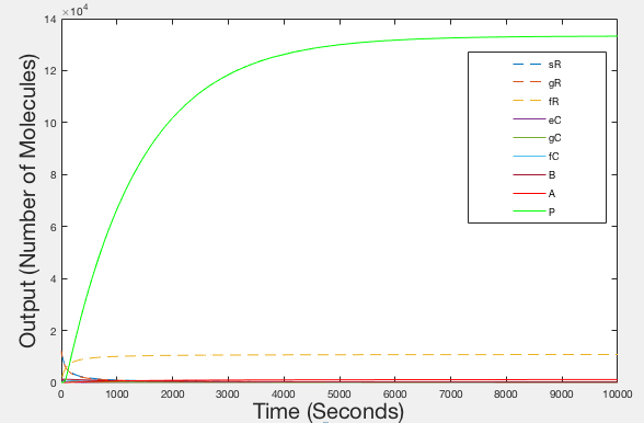
Figure 3: graph of Ideal Behaviour - Timespan 10000 seconds
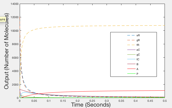
Figure 4: Graph of Realistic Behaviour - Timespan 0.5 seconds
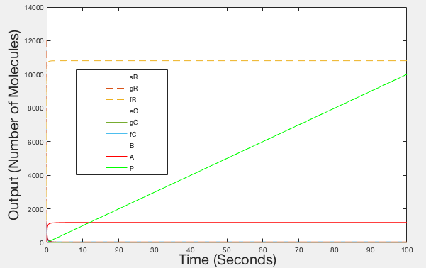
Figure 5: Graph of Realistic Behaviour - Timespan 100 seconds
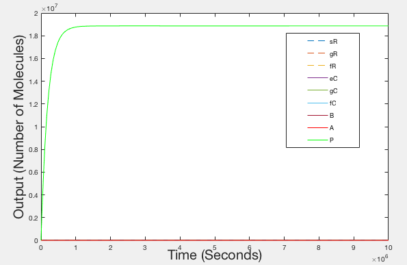
Figure 6: Graph of Realistic Behaviour - Timespan 10000000 seconds
How the Metal Aptamer System Works
A stunning testament to the modularity of our system is the fact that we could adapt it to also have the ability to detect metal ions in an environment. The sensing process would be slightly different but use of dCas9 would be the same.
At the start of the sensing process for metal ions, a folded sgRNA of our design will be present in abundance in the environment that we will be attempting to sense a metal ion within. These sgRNA molecules will have a dCAs9 handle incorporated onto them. Initially the sgRNA is folded in such a way that the dCas9 handle is obstructed by another part of the sgRNA molecule so the dCas9 molecule will be unable to bind.
The sgRNA molecules that we designed also have a site to which metal ions could bind to. So, in the presence of metal ions (Lead or Mercury) in the environment, the bonds in the ‘stem’ of the sgRNA are broken when the metal ions binds to the sgRNA site.
The bonds between the bases in the stem will then reform in different places, effectively extending the stem. With reformed, the dCas9 molecule will not be obstructed from binding to the dCas9 handle on the sgRNA. The process after this is the same as it would be for the sensing of Leptospirosis RNA.
Assumptions
- Binding strength of stem is the same when metal is and is not bound
- There is a possibility that other ions could bind to the same sgRNA, for simplicity, we assume that only one ion binds to one sgRNA at a time
- The stem will always bind back together after the bonds have initially broken
Having settled on a description of the process that our system would undertake, taking into account the stated assumptions, we proceeded to compose a reaction scheme. We achieved this by using our final reaction scheme for the Leptospirosis sensing system and altering the appropriate species in the reaction scheme. We used the reaction scheme to derive ODEs. As the system essentially works in the same way as our Leptospirosis system, the ODEs derived for our metal aptamer system were identical.
Explanation of Modelling Techniques Used
Shea Ackers Formalism
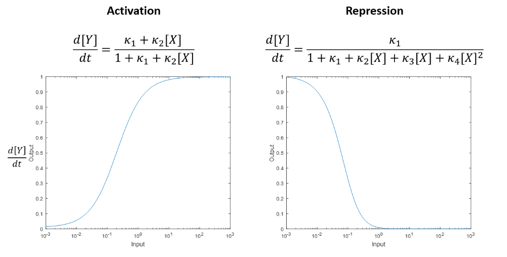
This is a method of gene regulation modelling. It is basically an extension of a Hill function. We are using the general equation for gene activation and adapting it with data specific to our research to model the production of GFP by our device. In figure 7, the general form of the Shea Ackers formalism is shown. The numerator represents all the states of our system where the gene is activated while the denominator represents all of the possible states that our system could be in (with their corresponding reaction constants). The graphs shows the sort of change in GFP production that we would expect to see with varying amounts of our activation complex present.
Mass Action Kinetics
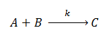
The law of mass action states that the rate of a chemical reaction is directly proportional to the product of the concentrations of the reactants. For example, an equation of the form:
Will yield the following ODEs representing the rate of change of the concentrations of the reactants:
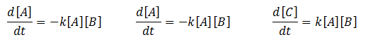
Where ‘k’ represents the association/dissociation constant of the reactants.
Hill Function
In most cases, the binding of a ligand to a molecule is aided when there are already other ligand present so the hill function is used to model gene regulation when there are already other ligands present (i.e. there is cooperative binding). It describes the percentage of a molecule already bound by ligand as a function of the ligand concentration. The following examples are general Hill function equations:
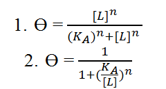
Key: n = hill coefficient, KA = Ligand concentration when half of binding sites are occupied by ligands, [L] = unbound ligand concentration, ϴ = Fraction of ligand binding sites on receiving molecule already occupied by ligands.
Equation 1 shows the form of the Hill function used when trying to model activation while equation 2 shows the form of the Hill function used for deactivation of genes. The hill function becomes a step function as the hill coefficient n → ∞.
Code
Code
Function dYdt = modelODE(T, Y, R, parameters);

%% modelODE
%
% ODEs of the system
%
%   dYdt = modelODE(T, Y, R, parameters)
%
%   Inputs
%       T and Y - current point utilized but the soler
%       R - anonymous function describing regulation of P production
%         - R must take the inputs R(gC, fC, A), in that order even if
%         values are unused
%       parameters - vector of parameters for mass action reactions
%

%% Explanation of the system
% Species
%   sR - RNA being sensed e.g. associated with Leptospirosis
%   gR - the guide RNA in the absence of the sR - this is a proxy specifies
%        representing the transcribed gRNA in its unfolded or partially folded
%        state
%   fR - guide RNA bound by sR
%   eC - the 'empty' Cas9 complex
%   gC - gR::eC complex - guide RNA in the absence of the sR bound to the
%        Cas9 complex. This complex can bind DNA (implications in promoter
%        regulation) but does not recruit RNA binding protein
%   fC - fR::eC complex - guide RNA in the presence of sR bound to Cas9
%        complex. This can bind DNA (implications in promoter regulation).
%        This can recruit RNA binding protein
%   B - RNA binding protein which activates transcription when targeted to
%       DNA
%   A - fR::eC::B complex - the complete activator which up regulates
%       protein output
%   P - Protein output
%
% Reactions
%
%   sR + gR -- af --> fR      fR -- ar --> sR + gR
%
%   gR + eC -- bf --> gC      gC -- br --> gR + eC
%
%   gC + sR -- gf --> fC      fC -- gr --> gC + sR
%
%   fR + eC -- df --> fC      fC -- dr --> fR + eC
%
%   fC +  B -- ef -->  A       A -- er --> fC +  B
%
%         0 -- R(gC,fC,A) --> P      P -- Delta --> 0
%
% Egheosa Ogbomo 2016-Aug-16
%

%% retrieve parameters
af = parameters(1);
ar = parameters(2);
bf = parameters(3);
br = parameters(4);
gf = parameters(5);
gr = parameters(6);
df = parameters(7);
dr = parameters(8);
ef = parameters(9);
er = parameters(10);
Delta = parameters(11);

%% retrieve current values
sR = Y(1);
gR = Y(2);
fR = Y(3);
eC = Y(4);
gC = Y(5);
fC = Y(6);
B = Y(7);
A = Y(8);
P = Y(9);

%% ODEs
dsRdt = - af.*sR.*gR + ar.*fR - gf.*gC.*sR + gr.*fC;

dgRdt = - af.*sR.*gR + ar.*fR - bf.*gR*eC + br.*gC;

dfRdt = + af.*sR.*gR - ar.*fR - df.*fR.*eC + dr.*fC;

deCdt = - bf.*gR.*eC + br.*gC - df.*fR.*eC + dr.*fC;

dgCdt = + bf.*gR.*eC - br.*gC - gf.*gC.*sR + gr.*fC;

dfCdt = + gf.*gC.*sR - gr.*fC + df.*fR.*eC - dr.*fC - ef.*fC.*B + er.*A;

dBdt = - ef.*fC.*B + er.*A;

dAdt = + ef.*fC.*B - er.*A;

dPdt = R(gC, fC, A) - Delta.*P;

%% return dYdt vector
dYdt = [dsRdt; dgRdt; dfRdt; deCdt; dgCdt; dfCdt; dBdt; dAdt; dPdt];

end

%% runModel
%
% Egheosa Ogbomo 2016-Aug-16
%

%% setup
clear all; close all;

%% specify regulatory mechanism
%
% Define an anonymous function which describes the regulation of the
% reporter gene promoter.
%
% Define an anonymous function in the following way (e.g. taking y = x^2 as
% an example)
%                          Y = @(X) X.^2
%
%                          Y(-2) = 4
%
% The anonymous function needs to take gC, fC and A as inputs (in
% that order).
%

% E.g. assume only A affects the promoter and that activation follows a
% Hill function:

alpha = 100; % production rate upon activation
n = 2; % Hill coefficient
kappa = 10; % dissociation constant

R = @(gC, fC, A) alpha.*(A.^n)./(kappa.^n + A.^n);

%% time span
tmax = 500;

%% initial conditions
sR0 = 12046; % RNA being sensed
gR0 = 12046; % unfolded nascent guide RNA - RNA state which binds C but not B
fR0 = 0; % folded guide RNA - which can recruit B to Cas9 complex
eC0 = 1204.6; % empty Cas9 complex
gC0 = 0; % Cas9:gR complex
fC0 = 0; % Cas9:fR complex
B0 = 1204.6; % RNA binding protein-RNAP fusion
A0 = 0; % Complete activator complex
P0 = 0; % Output protein e.g. GFP

%% parameters for binding reactions
af = 0.000001;
ar = 0.0000001;
bf = 0.000001;
br = 0.0000001;
gf = 0.000001;
gr = 0.0000001;
df = 0.000001;
dr = 0.0000001;
ef = 0.000001;
er = 0.0000001;
Delta = 0.00075;

%% simulate
[T,Y] = ode15s( @(T,Y) modelODE(T, Y, @(gC, fC, A) R(gC, fC, A), [af; ar; bf; br; gf; gr; df; dr; ef; er; Delta]), [0, tmax], [sR0; gR0; fR0; eC0; gC0; fC0; B0; A0; P0]);

%% retrieve results
sR = Y(:,1); gR = Y(:,2); fR = Y(:,3); eC = Y(:,4); gC = Y(:,5); fC = Y(:,6); B = Y(:,7); A = Y(:,8); P = Y(:,9);

%% plot
figure;
plot(T,sR,'--',T,gR,'--',T,fR,'--',T,eC,'-',T,gC,'-',T,fC,'-',T,B,'-',T,A,'-r',T,P,'-g')
legend('sR','gR','fR','eC','gC','fC','B','A','P');
xlabel('Time (Seconds)');
ylabel('Output (Number of Molecules)')