Difference between revisions of "Team:NCKU Tainan/Model Statistics Analysis"

In medicine, the blood glucose exceeding 5mM/L implies having diabetes, and it exceeding 120mM/L implies being a severe patient. Finding the person whose glucose concentration is over 5mM/L or 120mM/L is our target. First, we prove that there has difference between 0.1mM/L and 5mM/L (120mM/L) in the paired-difference T test part. And, we use the regression and prediction intervals to distinguish exceeding 120mM/L and 5mM/L from exceeding 0.1mM/L. From the result, 5mM/L can be distinguished from 0.1mM/L after 101 minutes, and 120mM/L can be distinguished from 0.1mM/L after 88 minutes.

In medicine, the blood glucose exceeding 5mM/L implies having diabetes, and it exceeding 120mM/L implies being a severe patient. Hence, we use paired-difference test to analyze whether the difference of these two groups (0.1 vs 5mM/L or 0.1 vs 120mM/L) have statistical significance in this part.

Procedure

1. Guessing that there is difference over 90 minutes, we analyze the data of 0.1mM/L and 5mM/L at 90 minutes first.

(Data)

Experiment Types	First	Second	...	Twelfth
0.1mM/L	358	368	...	338
5mM/L	369	386	...	385

Because the experiments of 0.1mM/L and 5mM/L have correlation and they are small sample, we choose the paired-difference test to examine whether there is difference in two groups at 90 minutes.

Analysis:
(use one-tailed test)

\(H_0:\mu_0\le0\ \ \ \ \ \ \ \ \ \ \ \ \ \ \ \ H_\alpha:\mu_0\ge0\)

Because the sample is small, we choose the t distribution to test.

d(=5mM/L-0.1mM/L)

11

18

...

47

\(n\) (Number of paired differences)=12
\(\bar{d}\) (Mean of the sample differences)= 26.16666667
\(s_d\) (Standard deviation of the sample differences) = \(\sqrt{\frac{\sum(d_i-\bar{d})^2}{n-1}}\) = 13.19664788

Test statistic t = \(\frac{\bar{d}-0}{s_d/\sqrt{n}}\) = 6.868713411 \(\gt t_{0.05,11}\) = 1.795885
P(t\(\gt\)6.868713411)= 1.995084e-05
Hence, We conclude that there is a difference between 0.1 and 5mM/L.

2. Find the minimal time at which there is statistical significance by paired-difference test.(use R program & α=0.05)

(Data)

Types Time(min)	0.1mM/L	...	0.1mM/L	5mM/L	...	5mM/L
0	295	...	276	292	...	291
1	296	...	276	290	...	291
2	301	...	277	292	...	287
. . .	. . .	...	. . .	. . .	...	. . .
119	392	...	372	420	...	443
120	392	...	374	427	...	439

By using R program
\(t_{0.05,11}\) = 1.795885

statistic Time(min)	T statistic (\(t_0\))
0	2.283227
1	1.992688
. . .	. . .
119	11.908155
120	15.538544

Hence, we can find \(t_0 \gt t_{0.05,11}\) at every time.

data0.1<-read.csv("C:/Users/Rick/Desktop/NCKUactivity/iGEM/819test/0.1urine.csv",header=T)
data5<-read.csv("C:/Users/Rick/Desktop/ NCKUactivity/iGEM/819test/5urine.csv",header=T)
difference<-cbind(data5[,2]-data0.1[,2],data5[,3]-data0.1[,3],data5[,4]-data0.1[,4],data5[,5]-data0.1[,5],data5[,6]-data0.1[,6],data5[,7]-data0.1[,7],data5[,8]-data0.1[,8],data5[,9]-data0.1[,9],data5[,10]-data0.1[,10],data5[,11]-data0.1[,11],data5[,12]-data0.1[,12],data5[,13]-data0.1[,13])
dbar<-difference%*% rep(1/12,12)
var<- ((difference -rep(dbar, 12))^2%*%rep(1,12))/11
sd<-var^0.5
t<-(dbar/sd)*(12^0.5)

3. Same with procedure 2, find the minimal time at which there is statistical significance by paired-difference test. (use R program, α=0.05, remove a outlier data)

By using R program
\(t_{0.05,10}\) = 1.812461

statistic Time(min)	T statistic (\(t_0\))
0	4.720629
1	4.580426
. . .	. . .
119	12.428324
120	14.240245

Hence, we can find \(t_0 \gt t_{0.05,10}\) at every time.

Conclusion:
        We can say there are the difference groups (0.1 vs 5 mM/L or 0.1 vs 120mM/L) in part 1 with the data. And then, we need to find an accurate value which can distinguish between two groups.

data0.1<-read.csv("C:/Users/Rick/Desktop/ NCKUactivity/iGEM/819test/0.1urine.csv",header=T)
data120<-read.csv("C:/Users/Rick/Desktop/ NCKUactivity/iGEM/819test/120urine.csv",header=T)
difference<-cbind(data120[,2]-data0.1[,2],data120[,3]-data0.1[,3],data120[,4]-data0.1[,4],data120[,5]-data0.1[,5],data120[,6]-data0.1[,6],data120[,8]-data0.1[,8],data120[,9]-data0.1[,9],data120[,10]-data0.1[,10],data120[,11]-data0.1[,11],data120[,12]-data0.1[,12],data120[,13]-data0.1[,13])
dbar<-difference%*% rep(1/11,11)
var<- ((difference -rep(dbar, 11))^2%*%rep(1,11))/10
sd<-var^0.5
t<-(dbar/sd)*(11^0.5)

        Our product uses the fluorescence intensity to obtain the concentration of blood glucose. Therefore, whether we could precisely distinguish exceeding 120mM/L and 5mM/L from exceeding 0.1mM/L becomes the most important problem. We use the skill of the prediction interval in this part.

Procedure

1. Use the regression to find the model of 0.1, 5, 120mM/L, and show the prediction interval plot.

(0.1mM/L)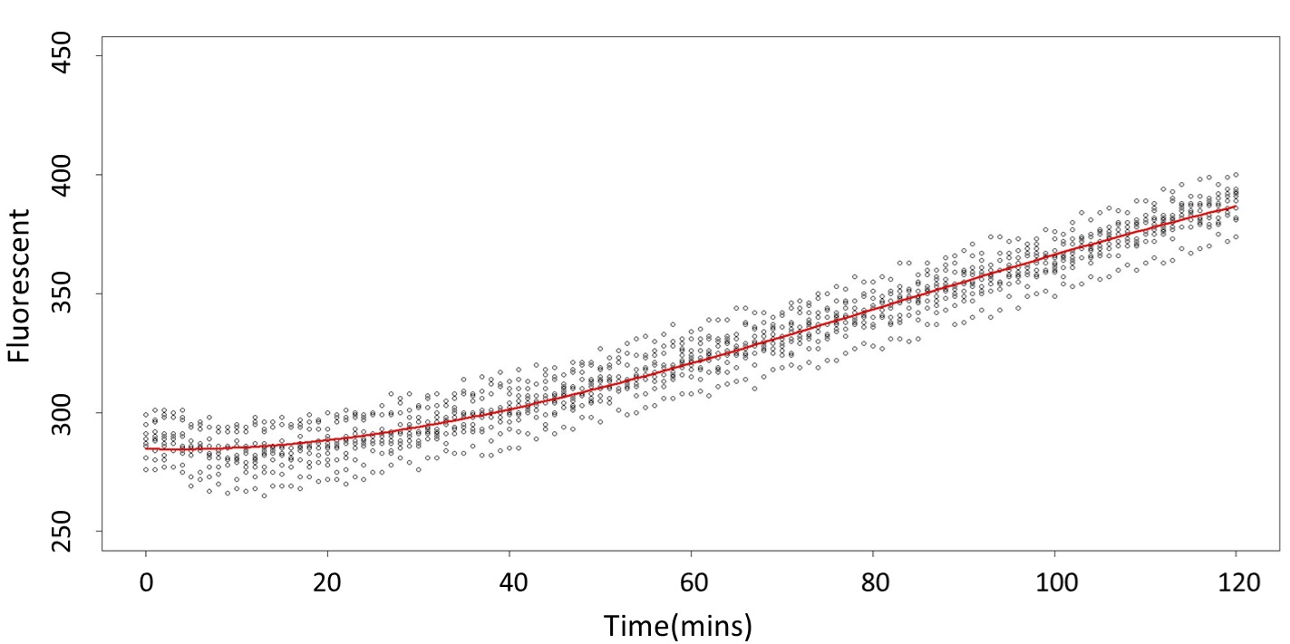

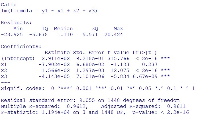
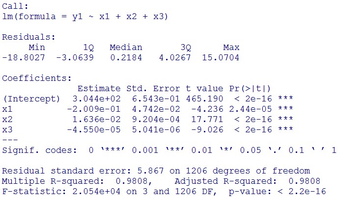
(summary)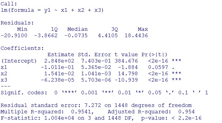

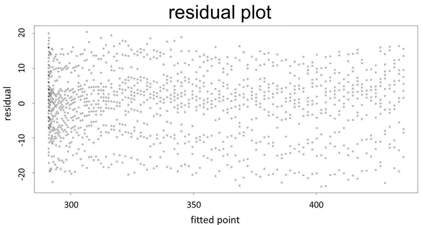
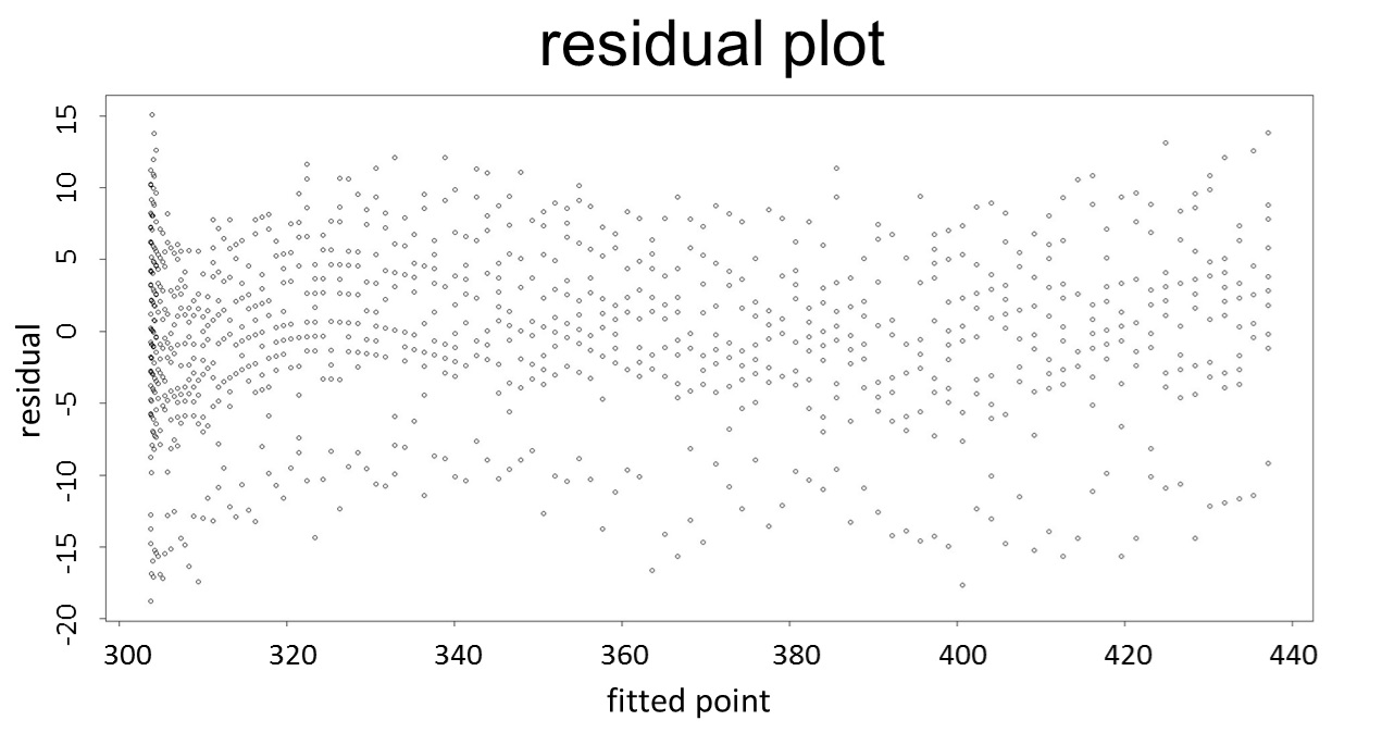
(residual plot)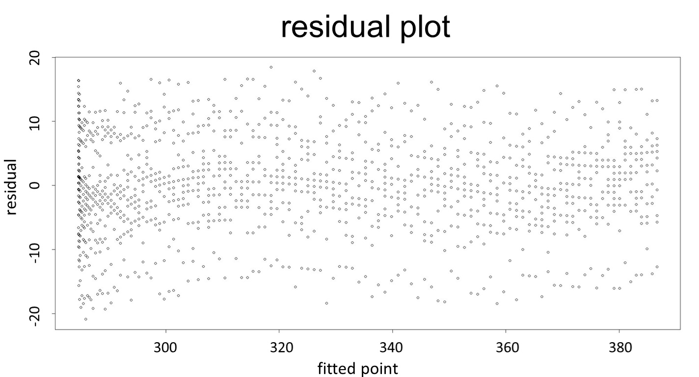

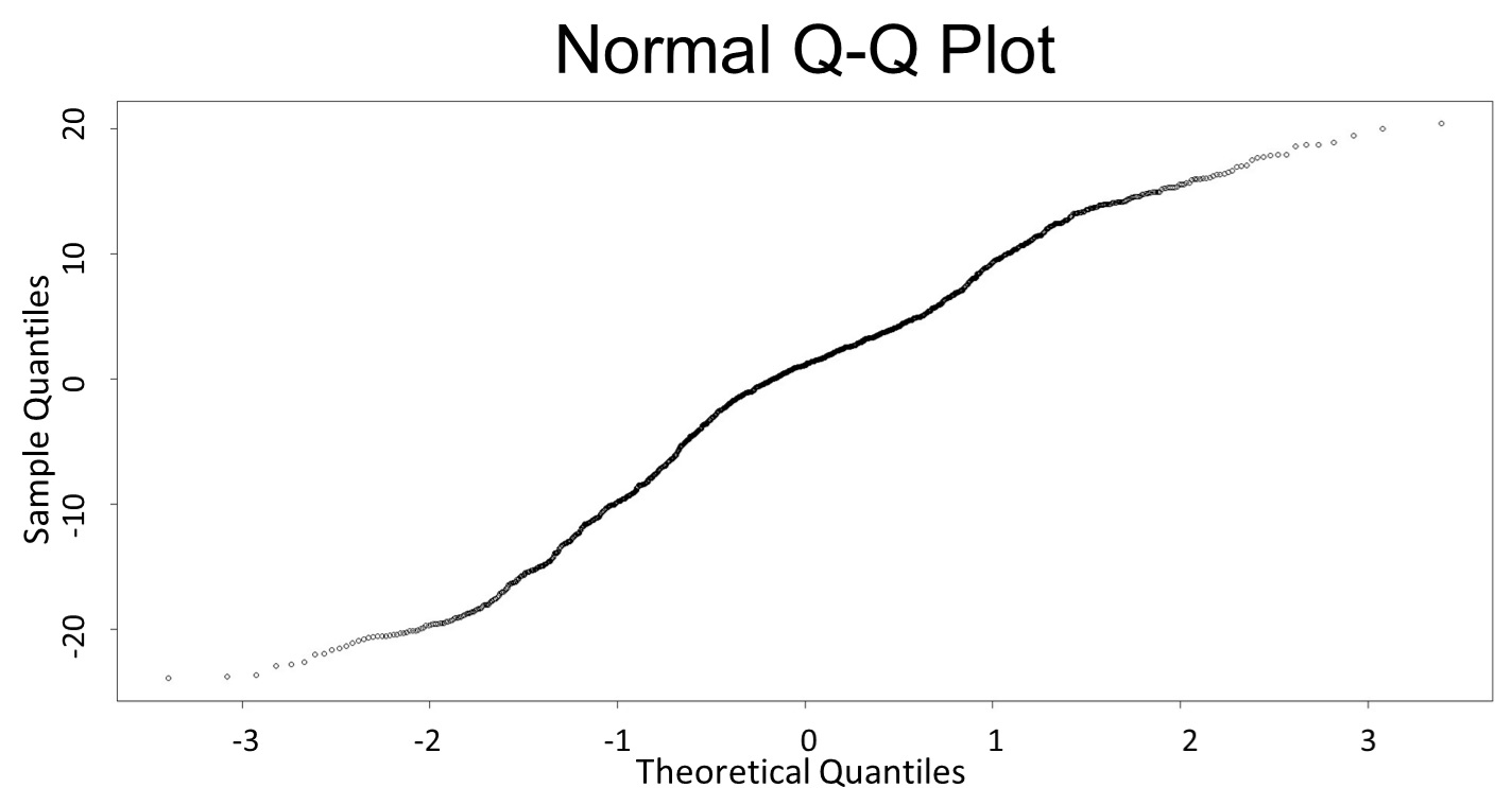
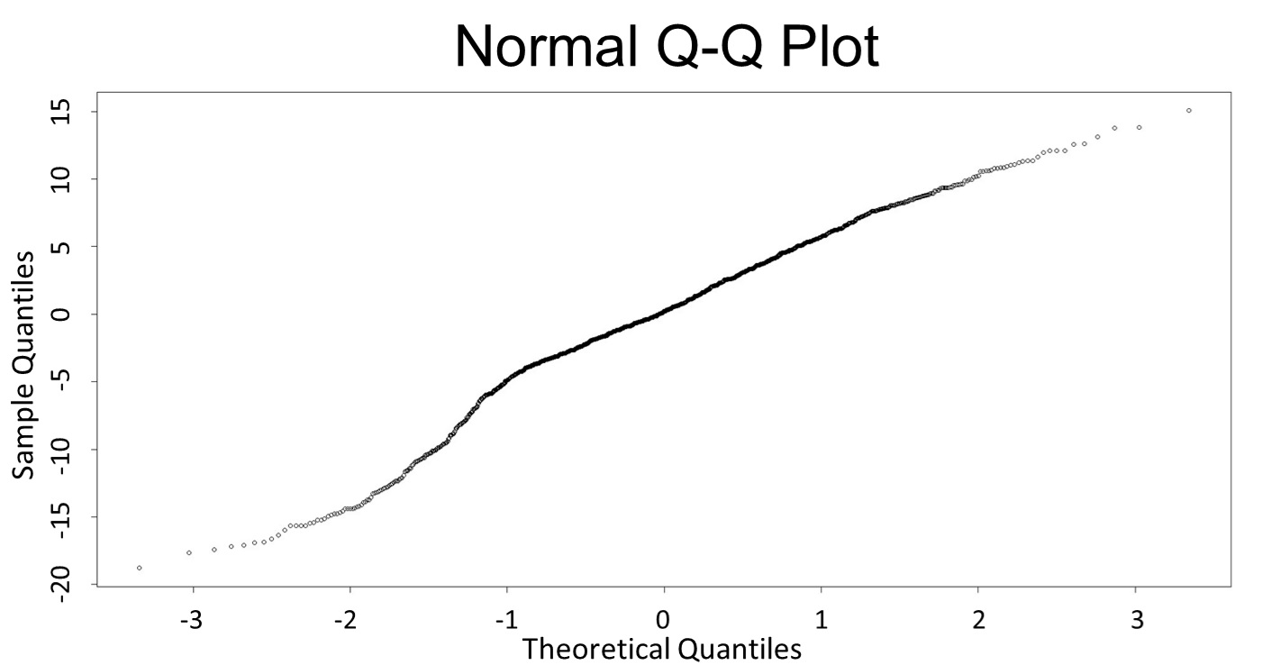
(Q-Q plot)

This model conforms the assumption and R-square is equal to 0.9541, so we think the cubic polynomial regression model is suitable.

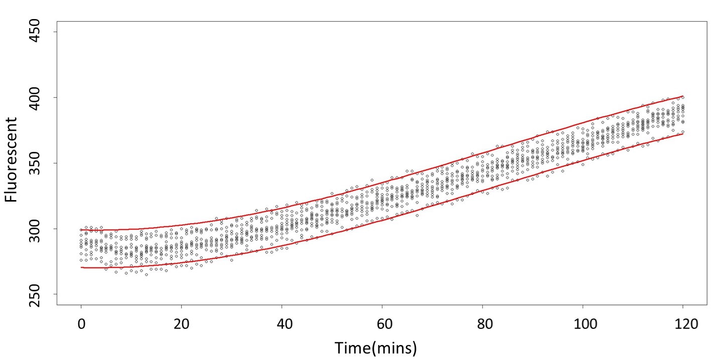
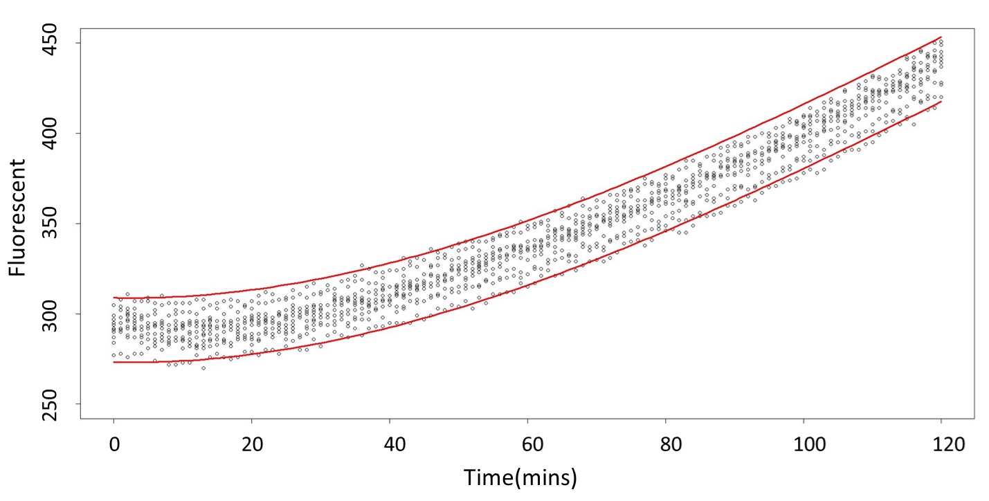
(prediction interval)
Formula: \(\bar{X}\pm t_{\frac{\alpha}{2},n-1}S\sqrt{1+\frac{1}{n}}\)

And look the following, the procedure is same in the 5mM/L and 120mM/L.

(5mM/L)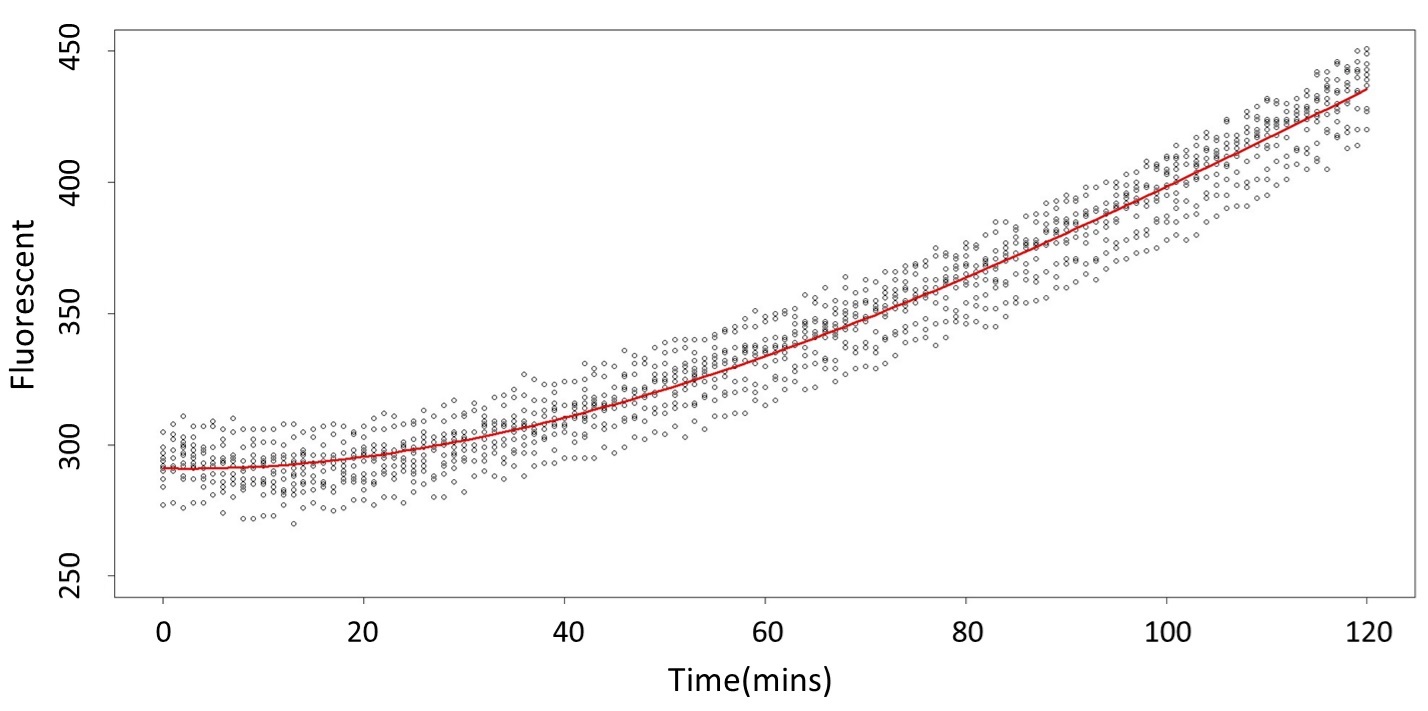(120mM/L)

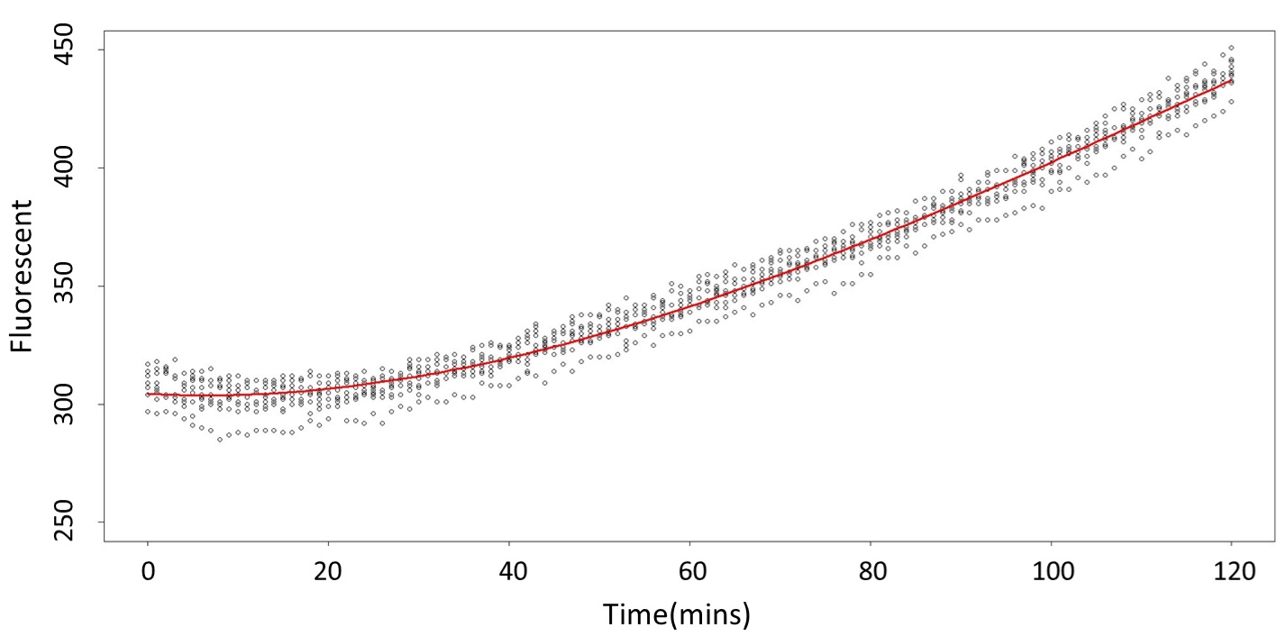
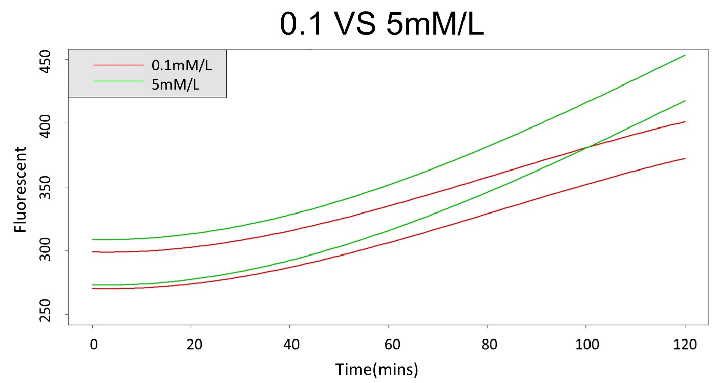
2. According to the previous part, we can say that 0.1mM/L and 5mM/L are difference group by the statistical significance. In order to precisely distinguish these two groups, choose the time at which the 5mmo/L and 0.1mmo/L prediction interval started to diverge to be the recommended prediction time.

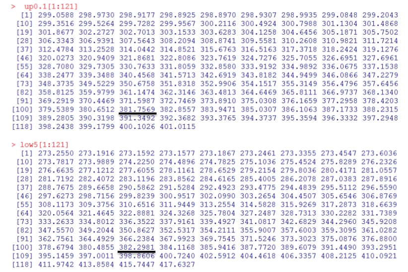
By the above tables, we can see that 5mM/L low prediction line exceeds 0.1mM/L up prediction line when the time is more than 101 mins. Hence, it can be expected to have a higher accuracy to take the data after 101 mins.

(prediction interval of 0.1 &5 mM/L)

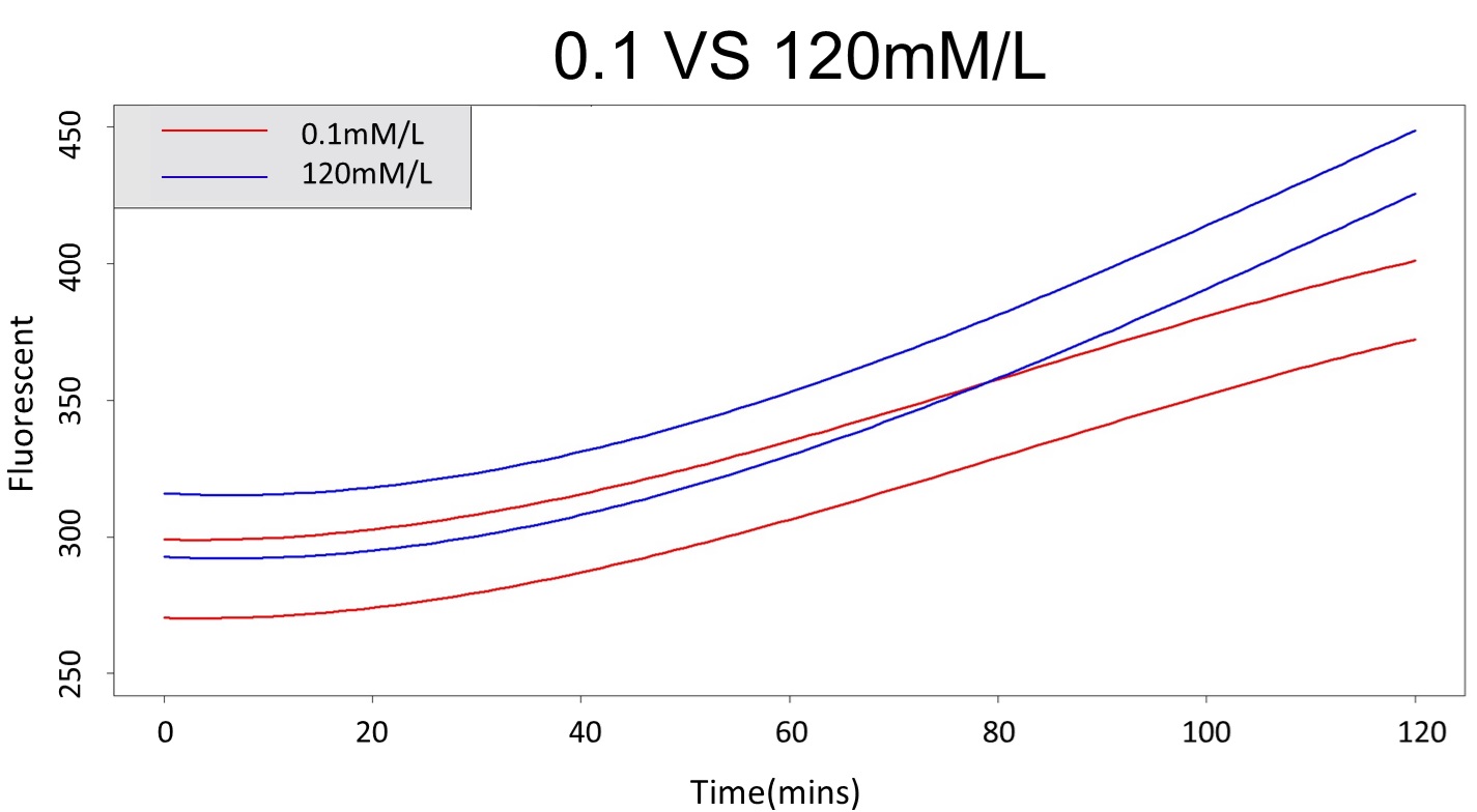
3. Same with procedure 2, choose the time at which the 120mmo/L and 0.1mmo/L prediction interval started to diverge to be the recommended prediction time.

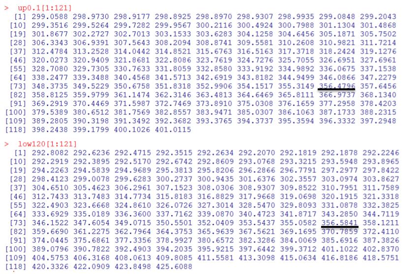
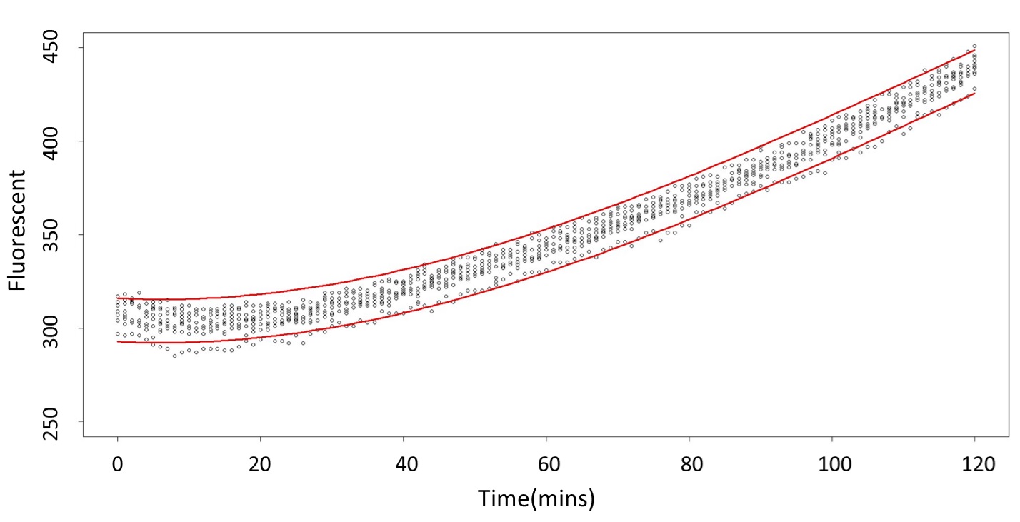
By the above tables, we can find that 120mM/L low prediction line exceeds 0.1mM/L up prediction line when the time is more than 88 mins. Hence, it can be expected to have a higher accuracy to take the data in 88 mins.

(prediction interval of 0.1 &120 mM/L)

#0.1 vs 5
#0.1 urine plot
data<-read.csv("C:/Users/Rick/Desktop/NCKUactivity/iGEM/819test/0.1urine.csv",header=T)
x1<-rep(data[,1],12)
x2<-x1^2
x3<-x1^3
y1<-c(data[,2],data[,3],data[,4],data[,5],data[,6],data[,7], data[,8],data[,9],data[,10], data[,11],data[,12],data[,13])
model<-lm(y1~x1+x2+x3)
yhat0.1<-model$fit
plot(x1,y1,ylim=c(250,450),xlab= "time(mins) ",ylab= "Fluorescent", cex.lab=1.5)
#lines(data[,1], yhat0.1[1:121],lwd=3,col=2)
n=121*12 
mse<-sum((y1-yhat0.1)^2)/(n-3)  # calculate MS_Res(=σ^2)
X<-cbind(1,x1,x2,x3)
se<-sqrt(mse*(1+X[1,]%*%solve(t(X)%*%X)%*%X[1,]))
up0.1<-model$coefficients[1]+x1*model$coefficients[2]+x2*model$coefficients[3]+x3*model$coefficients[4]+qt(.975,df=n-2)*se
low0.1<-model$coefficients[1]+x1*model$coefficients[2]+x2*model$coefficients[3]+x3*model$coefficients[4]+qt(.025,df=n-2)*se
lines(data[,1], up0.1[1:121], col=2,lwd=3)
lines(data[,1], low0.1[1:121],col=2,lwd=3)
#5 urine plot
data<-read.csv("C:/Users/Rick/Desktop/NCKUactivity/iGEM/819test/5urine.csv",header=T)
x1<-rep(data[,1],12)
x2<-x1^2
x3<-x1^3
y1<-c(data[,2],data[,3],data[,4],data[,5],data[,6],data[,7], data[,8],data[,9],data[,10], data[,11],data[,12],data[,13])
model<-lm(y1~x1+x2+x3)
yhat5<-model$fit 
par(new=TRUE)
plot(x1,y1,ylim=c(250,450),xlab= "time(mins) ",ylab= "Fluorescent", cex.lab=1.5)
#lines(data[,1], yhat5[1:121],lwd=3,col=2)
n=121*12 
mse<-sum((y1-yhat5)^2)/(n-3)  # calculate MS_Res(=σ^2)
X<-cbind(1,x1,x2,x3)
se<-sqrt(mse*(1+X[1,]%*%solve(t(X)%*%X)%*%X[1,]))
up5<-model$coefficients[1]+x1*model$coefficients[2]+x2*model$coefficients[3]+x3*model$coefficients[4]+qt(.975,df=n-2)*se
low5<-model$coefficients[1]+x1*model$coefficients[2]+x2*model$coefficients[3]+x3*model$coefficients[4] +qt(.025,df=n-2)*se
lines(data[,1], up5[1:121], col=3,lwd=3)
lines(data[,1], low5[1:121], col=3,lwd=3)
title(main="0.1 vs 5mM/L",cex.main=4)
Name<-c(expression(paste("0.1mM/L")),expression(paste("5mM/L")))
legend("topleft", Name, ncol = 1, cex = 1.5, col=c("red","green"),lwd = c(2,2), bg = 'gray90')
#0.1 vs 120
#0.1 urine plot
data<-read.csv("C:/Users/Rick/Desktop/NCKUactivity/iGEM/819test/0.1urine.csv",header=T)
x1<-rep(data[,1],12)
x2<-x1^2
x3<-x1^3
y1<-c(data[,2],data[,3],data[,4],data[,5],data[,6],data[,7], data[,8],data[,9],data[,10], data[,11],data[,12],data[,13])
model<-lm(y1~x1+x2+x3)
yhat0.1<-model$fit
plot(x1,y1,ylim=c(250,450),xlab= "time(mins) ",ylab= "Fluorescent", cex.lab=1.5)
#lines(data[,1], yhat0.1[1:121],lwd=3,col=2)
n=121*12 
mse<-sum((y1-yhat0.1)^2)/(n-3)  # calculate MS_Res(=σ^2)
X<-cbind(1,x1,x2,x3)
se<-sqrt(mse*(1+X[1,]%*%solve(t(X)%*%X)%*%X[1,]))
up0.1<-model$coefficients[1]+x1*model$coefficients[2]+x2*model$coefficients[3]+x3*model$coefficients[4]+qt(.975,df=n-2)*se
low0.1<-model$coefficients[1]+x1*model$coefficients[2]+x2*model$coefficients[3]+x3*model$coefficiens[4]+qt(.025,df=n-2)*se
lines(data[,1], up0.1[1:121], col=2,lwd=3)
lines(data[,1], low0.1[1:121],col=2,lwd=3)
#120 urine plot
data<-read.csv("C:/Users/Rick/Desktop/NCKUactivity/iGEM/819test/120urine.csv",header=T)
x1<-rep(data[,1],10)
x2<-x1^2
x3<-x1^3
y1<-c(data[,2],data[,3],data[,4],data[,5],data[,6],data[,9],data[,10],data[,11],data[,12],data[,13])
model<-lm(y1~x1+x2+x3)
yhat120<-model$fit 
par(new=TRUE)
plot(x1,y1,ylim=c(250,450),xlab= "time(mins) ",ylab= "Fluorescent", cex.lab=1.5)
#lines(data[,1], yhat120[1:121],lwd=3,col=2)
n=121*10 
mse<-sum((y1-yhat120)^2)/(n-3)  # calculate MS_Res(=σ^2)
X<-cbind(1,x1,x2,x3)
se<-sqrt(mse*(1+X[1,]%*%solve(t(X)%*%X)%*%X[1,]))
up120<-model$coefficients[1]+x1*model$coefficients[2]+x2*model$coefficients[3]+x3*model$coefficients[4]+qt(.975,df=n-2)*se
low120<-model$coefficients[1]+x1*model$coefficients[2]+x2*model$coefficients[3]+x3*model$coefficients[4]+qt(.025,df=n-2)*se
lines(data[,1], up120[1:121], col=4,lwd=3)
lines(data[,1], low120[1:121], col=4,lwd=3)
title(main="0.1 vs 120mM/L",cex.main=4)
Name<-c(expression(paste("0.1mM/L")),expression(paste("120mM/L")))
legend("topleft", Name, ncol = 1, cex = 1.5, col=c("red","green"),lwd = c(2,2), bg = 'gray90')

• Introduction
• Paired-difference T test
• Regression & Prediction
• Appendix