Difference between revisions of "Team:NCKU Tainan/Model Statistics Analysis"
| Line 13: | Line 13: | ||
<div class="head2">Model: Statistics Analysis</div> | <div class="head2">Model: Statistics Analysis</div> | ||
<div class="title-line" id="intro">Introduction</div> | <div class="title-line" id="intro">Introduction</div> | ||
| − | <p>In medicine, when the presence of urine glucose exceeds | + | <p>In medicine, when the presence of urine glucose exceeds 5 mM, it implies pre-diabetes or diabetes. However, we refer to people whose urine glucose exceeds 120 mM as sever diabetic patients. Consequently, finding the person whose urine glucose concentration is over 5 mM or 120 mM is our target for prevention and early detection.</p> |
| − | <p>First, we prove that there is a difference between 0. | + | <p>First, we prove that there is a difference between 0.1 mM and 5 mM (120 mM) in the <a href="#pair" onclick="return toEvent('pair');">paired-difference T test</a> part. And, we use the <a href="#reg" onclick="return toEvent('reg');">regression and prediction intervals</a> to distinguish exceeding 120 mM and 5 mM from exceeding 0.1 mM. From the result, 5 mM can be distinguished from 0.1 mM after 101 minutes, and 120 mM can be distinguished from 0.1 mM after 88 minutes.</p> |
<img src="/wiki/images/c/c0/T--NCKU_Tainan--project-modeling-statistic-image1.jpg"> | <img src="/wiki/images/c/c0/T--NCKU_Tainan--project-modeling-statistic-image1.jpg"> | ||
<img src="/wiki/images/0/04/T--NCKU_Tainan--project-modeling-statistic-image2.jpg"> | <img src="/wiki/images/0/04/T--NCKU_Tainan--project-modeling-statistic-image2.jpg"> | ||
<div class="title-line long" id="pair"></div> | <div class="title-line long" id="pair"></div> | ||
<div class="title-content">Paired-difference T test</div> | <div class="title-content">Paired-difference T test</div> | ||
| − | <p>In medicine, the urine glucose exceeds | + | <p>In medicine, the urine glucose exceeds 5 mM implies having diabetes, and it exceeding 120 mM implies being a severe patient. Hence, we use paired-difference test to analyze whether the difference of these two groups (0.1 vs 5 mM or 0.1 vs 120 mM) have statistical significance in this part.</p> |
<br><br> | <br><br> | ||
<p>Procedure</p> | <p>Procedure</p> | ||
<br> | <br> | ||
| − | <p>1. Predicting if there is a difference over 90 minutes, we analyze the data of 0. | + | <p>1. Predicting if there is a difference over 90 minutes, we analyze the data of 0.1 mM and 5 mM at 90 minutes first.</p> |
<p>(Data)</p> | <p>(Data)</p> | ||
<table> | <table> | ||
| Line 34: | Line 34: | ||
</tr> | </tr> | ||
<tr> | <tr> | ||
| − | <td>0. | + | <td>0.1 mM</td> |
<td>358</td> | <td>358</td> | ||
<td>368</td> | <td>368</td> | ||
| Line 41: | Line 41: | ||
</tr> | </tr> | ||
<tr> | <tr> | ||
| − | <td> | + | <td>5 mM</td> |
<td>369</td> | <td>369</td> | ||
<td>386</td> | <td>386</td> | ||
| Line 49: | Line 49: | ||
</tbody></table> | </tbody></table> | ||
<br> | <br> | ||
| − | <p>Because the experiments of 0. | + | <p>Because the experiments of 0.1 mM and 5 mM have correlation and they are small sample, we choose the paired-difference test to examine whether there is difference in two groups at 90 minutes.</p> |
<br> | <br> | ||
<p>Analysis:<br>(use one-tailed test)<br></p> | <p>Analysis:<br>(use one-tailed test)<br></p> | ||
| Line 56: | Line 56: | ||
<table> | <table> | ||
<tbody><tr> | <tbody><tr> | ||
| − | <td class="size1">d(= | + | <td class="size1">d(= 5 mM - 0.1 mM)</td> |
<td class="size2">11</td> | <td class="size2">11</td> | ||
<td class="size2">18</td> | <td class="size2">18</td> | ||
| Line 64: | Line 64: | ||
</tbody></table> | </tbody></table> | ||
<p>\(n\) (Number of paired differences)=12<br>\(\bar{d}\) (Mean of the sample differences)= 26.16666667<br>\(s_d\) (Standard deviation of the sample differences) = \(\sqrt{\frac{\sum(d_i-\bar{d})^2}{n-1}}\) = 13.19664788</p> | <p>\(n\) (Number of paired differences)=12<br>\(\bar{d}\) (Mean of the sample differences)= 26.16666667<br>\(s_d\) (Standard deviation of the sample differences) = \(\sqrt{\frac{\sum(d_i-\bar{d})^2}{n-1}}\) = 13.19664788</p> | ||
| − | <p>Test statistic t = \(\frac{\bar{d}-0}{s_d/\sqrt{n}}\) = 6.868713411 \(\gt t_{0.05,11}\) = 1.795885<br>P(t\(\gt\)6.868713411)= 1.995084e-05<br>Hence, we conclude that there is a difference between 0.1 and | + | <p>Test statistic t = \(\frac{\bar{d}-0}{s_d/\sqrt{n}}\) = 6.868713411 \(\gt t_{0.05,11}\) = 1.795885<br>P(t\(\gt\)6.868713411)= 1.995084e-05<br>Hence, we conclude that there is a difference between 0.1 and 5 mM.</p> |
<p>2. Find the minimal time at which there is statistical significance by paired-difference test.(use R program & α=0.05)</p> | <p>2. Find the minimal time at which there is statistical significance by paired-difference test.(use R program & α=0.05)</p> | ||
<p>(Data)</p> | <p>(Data)</p> | ||
| Line 70: | Line 70: | ||
<tbody><tr> | <tbody><tr> | ||
<th class="size1 dial"><div class="right">Types</div><br><div class="left">Time(min)</div></th> | <th class="size1 dial"><div class="right">Types</div><br><div class="left">Time(min)</div></th> | ||
| − | <th class="size2">0. | + | <th class="size2">0.1 mM</th> |
<th class="size3">...</th> | <th class="size3">...</th> | ||
| − | <th class="size2">0. | + | <th class="size2">0.1 mM</th> |
| − | <th class="size2"> | + | <th class="size2">5 mM</th> |
<th class="size3">...</th> | <th class="size3">...</th> | ||
| − | <th class="size2"> | + | <th class="size2">5 mM</th> |
</tr> | </tr> | ||
<tr> | <tr> | ||
| Line 197: | Line 197: | ||
</tbody></table> | </tbody></table> | ||
<p>Hence, we can find \(t_0 \gt t_{0.05,10}\) at every time.</p> | <p>Hence, we can find \(t_0 \gt t_{0.05,10}\) at every time.</p> | ||
| − | <p>Conclusion:<br> We can say there are the differet groups (0.1 vs 5 mM or 0.1 vs | + | <p>Conclusion:<br> We can say there are the differet groups (0.1 vs 5 mM or 0.1 vs 120 mM) in part 1 with the data. And then, we need to find an accurate value which can distinguish between two groups.</p> |
<pre><code class="R">data0.1<-read.csv("C:/Users/Rick/Desktop/ NCKUactivity/iGEM/819test/0.1urine.csv",header=T) | <pre><code class="R">data0.1<-read.csv("C:/Users/Rick/Desktop/ NCKUactivity/iGEM/819test/0.1urine.csv",header=T) | ||
data120<-read.csv("C:/Users/Rick/Desktop/ NCKUactivity/iGEM/819test/120urine.csv",header=T) | data120<-read.csv("C:/Users/Rick/Desktop/ NCKUactivity/iGEM/819test/120urine.csv",header=T) | ||
| Line 207: | Line 207: | ||
<div class="title-line long" id="reg"></div> | <div class="title-line long" id="reg"></div> | ||
<div class="title-content">Regression & Prediction interval [1]</div> | <div class="title-content">Regression & Prediction interval [1]</div> | ||
| − | <p> Our product uses the fluorescence intensity to obtain the concentrations of urine glucose. According to our results, we precisely distinguished the concentrations of | + | <p> Our product uses the fluorescence intensity to obtain the concentrations of urine glucose. According to our results, we precisely distinguished the concentrations of 5 mM and 120 mM from 0.1 mM by using fluorescence intensity with 99% accuracy. Consequently, we use the skill of the prediction interval in this part.</p> |
<br> | <br> | ||
<p>Procedure</p> | <p>Procedure</p> | ||
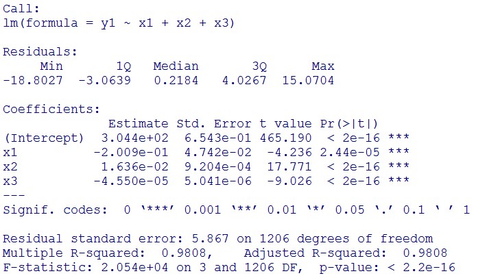
| − | <p>1. Use the regression to find the model of 0.1, 5, | + | <p>1. Use the regression to find the model of 0.1, 5, 120 mM, and show the prediction interval plot.</p> |
| − | <p class="center">(0. | + | <p class="center">(0.1 mM)<img src="/wiki/images/a/a3/T--NCKU_Tainan--project-modeling-statistic-image3.jpg"></p> |
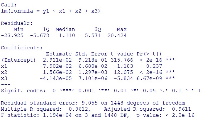
<p>(summary)<img src="/wiki/images/5/5e/T--NCKU_Tainan--project-modeling-statistic-image4.jpg"></p> | <p>(summary)<img src="/wiki/images/5/5e/T--NCKU_Tainan--project-modeling-statistic-image4.jpg"></p> | ||
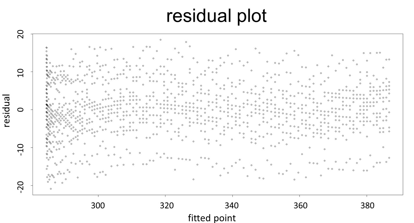
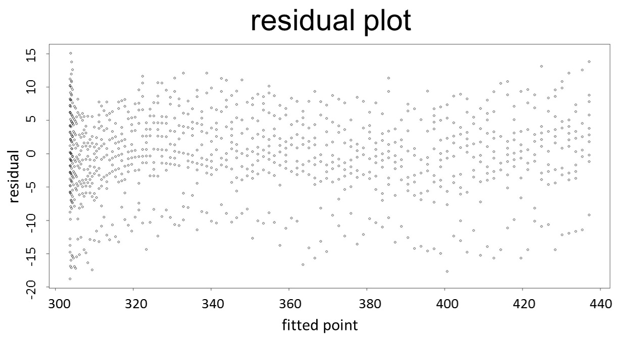
<p>(residual plot) [2]</p> | <p>(residual plot) [2]</p> | ||
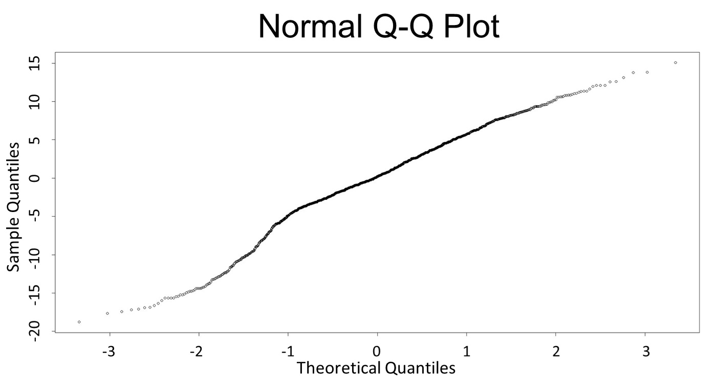
| Line 220: | Line 220: | ||
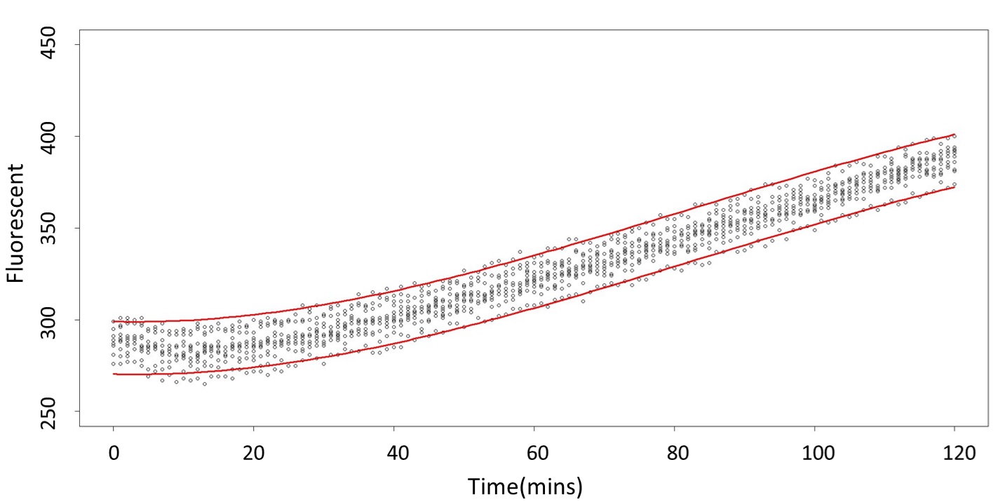
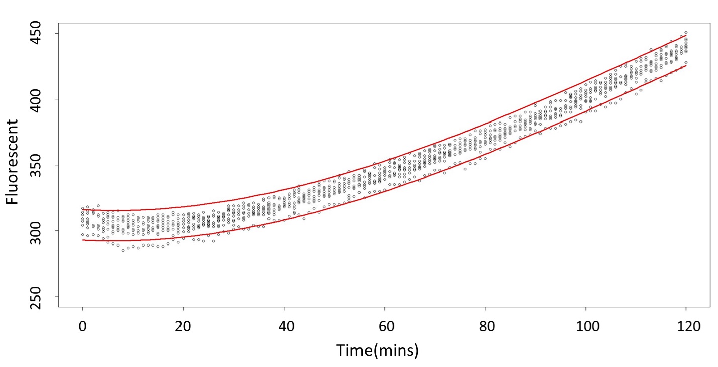
<p>(prediction interval)<br>Formula: \(\bar{X}\pm t_{\frac{\alpha}{2},n-1}S\sqrt{1+\frac{1}{n}}\)</p> | <p>(prediction interval)<br>Formula: \(\bar{X}\pm t_{\frac{\alpha}{2},n-1}S\sqrt{1+\frac{1}{n}}\)</p> | ||
<img src="/wiki/images/5/5e/T--NCKU_Tainan--project-modeling-statistic-image7.jpg"> | <img src="/wiki/images/5/5e/T--NCKU_Tainan--project-modeling-statistic-image7.jpg"> | ||
| − | <p>And the procedure is same in the | + | <p>And the procedure is same in the 5 mM and 120 mM.</p><p class="center">(5 mM)<img src="/wiki/images/b/b4/T--NCKU_Tainan--project-modeling-statistic-image8.jpg"><img src="/wiki/images/6/69/T--NCKU_Tainan--project-modeling-statistic-image9.jpg"><img src="/wiki/images/c/c9/T--NCKU_Tainan--project-modeling-statistic-image10.jpg"><img src="/wiki/images/b/b6/T--NCKU_Tainan--project-modeling-statistic-image11.jpg"><img src="/wiki/images/f/ff/T--NCKU_Tainan--project-modeling-statistic-image12.jpg">(120 mM)<img src="/wiki/images/8/84/T--NCKU_Tainan--project-modeling-statistic-image13.jpg"><img src="/wiki/images/a/a5/T--NCKU_Tainan--project-modeling-statistic-image14.jpg"><img src="/wiki/images/0/09/T--NCKU_Tainan--project-modeling-statistic-image15.jpg"><img src="/wiki/images/e/ef/T--NCKU_Tainan--project-modeling-statistic-image16.jpg"><img src="/wiki/images/f/f1/T--NCKU_Tainan--project-modeling-statistic-image17.jpg"></p> |
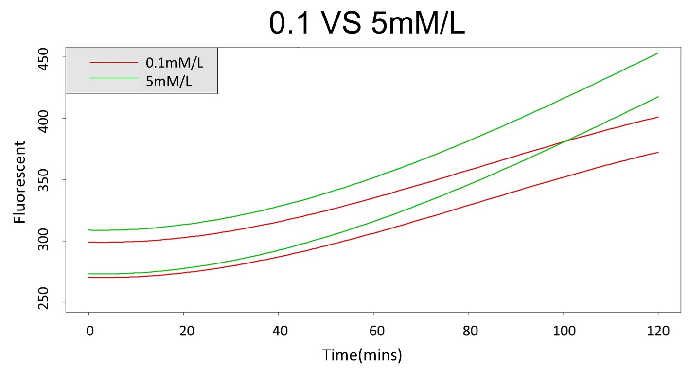
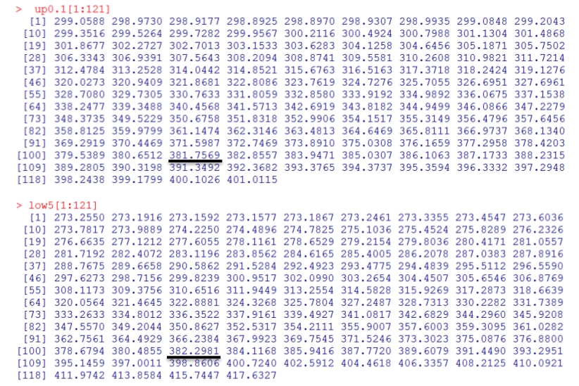
| − | <p>2. According to the <a href="#pair" onclick="return toEvent('pair');">paired-difference T test</a> part, it demonstrates that 0. | + | <p>2. According to the <a href="#pair" onclick="return toEvent('pair');">paired-difference T test</a> part, it demonstrates that 0.1 mM and 5 mM can be identified as different group due to the statistical significance. In order to precisely distinguish these two groups, choose the time at which the 5 mM and 0.1 mM prediction interval started to diverge to be the recommended prediction time.</p><img src="/wiki/images/e/ec/T--NCKU_Tainan--project-modeling-statistic-image18.jpg"> |
<p>Based on the above tables, it showed a significant degree of accuracy when an intersection upon the maximum fluorescence intensity at 0.1 mM and the minimum fluorescence intensity at 5 mM occurs after 101 mins (t> 101 mins). Hence, it can be expected to have higher accuracy of data after 101 mins.</p> | <p>Based on the above tables, it showed a significant degree of accuracy when an intersection upon the maximum fluorescence intensity at 0.1 mM and the minimum fluorescence intensity at 5 mM occurs after 101 mins (t> 101 mins). Hence, it can be expected to have higher accuracy of data after 101 mins.</p> | ||
<br> | <br> | ||
<p>(prediction interval of 0.1 &5 mM)</p> | <p>(prediction interval of 0.1 &5 mM)</p> | ||
<img src="/wiki/images/c/c0/T--NCKU_Tainan--project-modeling-statistic-image1.jpg"> | <img src="/wiki/images/c/c0/T--NCKU_Tainan--project-modeling-statistic-image1.jpg"> | ||
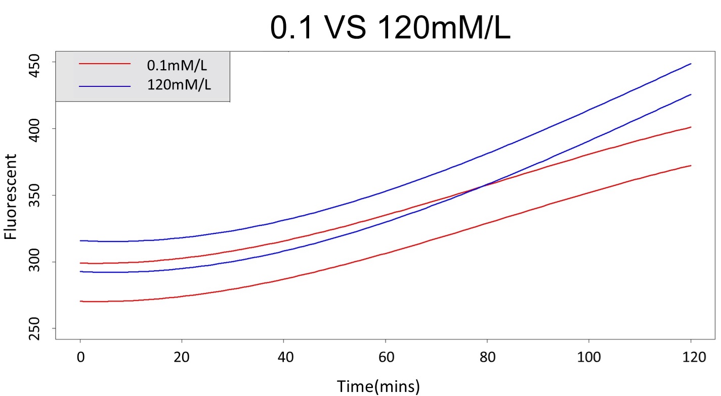
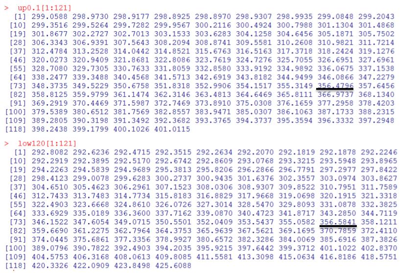
| − | <p>3. As same as Procedure 2, we choose the time at | + | <p>3. As same as Procedure 2, we choose the time at 120 mM and 0.1 mM prediction interval to diverge to be the recommended prediction </p> |
<img src="/wiki/images/b/b9/T--NCKU_Tainan--project-modeling-statistic-image19.jpg"> | <img src="/wiki/images/b/b9/T--NCKU_Tainan--project-modeling-statistic-image19.jpg"> | ||
<p>According to the above tables, it showed a significant degree of accuracy when an intersection upon the maximum fluorescence intensity at 5 mM and minimum fluorescence intensity at 120 mM occurs after 88 mins (t> 88 mins). Hence, it can be expected to have higher accuracy of data after 88 mins.</p> | <p>According to the above tables, it showed a significant degree of accuracy when an intersection upon the maximum fluorescence intensity at 5 mM and minimum fluorescence intensity at 120 mM occurs after 88 mins (t> 88 mins). Hence, it can be expected to have higher accuracy of data after 88 mins.</p> | ||
Latest revision as of 16:09, 19 October 2016
In medicine, when the presence of urine glucose exceeds 5 mM, it implies pre-diabetes or diabetes. However, we refer to people whose urine glucose exceeds 120 mM as sever diabetic patients. Consequently, finding the person whose urine glucose concentration is over 5 mM or 120 mM is our target for prevention and early detection.
First, we prove that there is a difference between 0.1 mM and 5 mM (120 mM) in the paired-difference T test part. And, we use the regression and prediction intervals to distinguish exceeding 120 mM and 5 mM from exceeding 0.1 mM. From the result, 5 mM can be distinguished from 0.1 mM after 101 minutes, and 120 mM can be distinguished from 0.1 mM after 88 minutes.
In medicine, the urine glucose exceeds 5 mM implies having diabetes, and it exceeding 120 mM implies being a severe patient. Hence, we use paired-difference test to analyze whether the difference of these two groups (0.1 vs 5 mM or 0.1 vs 120 mM) have statistical significance in this part.
Procedure
1. Predicting if there is a difference over 90 minutes, we analyze the data of 0.1 mM and 5 mM at 90 minutes first.
(Data)
Experiment Types |
First | Second | ... | Twelfth |
|---|---|---|---|---|
| 0.1 mM | 358 | 368 | ... | 338 |
| 5 mM | 369 | 386 | ... | 385 |
Because the experiments of 0.1 mM and 5 mM have correlation and they are small sample, we choose the paired-difference test to examine whether there is difference in two groups at 90 minutes.
Analysis:
(use one-tailed test)
\(H_0:\mu_0\le0\ \ \ \ \ \ \ \ \ \ \ \ \ \ \ \ H_\alpha:\mu_0\ge0\)
Because the sample is small, we choose the t distribution to test.
| d(= 5 mM - 0.1 mM) | 11 | 18 | ... | 47 |
\(n\) (Number of paired differences)=12
\(\bar{d}\) (Mean of the sample differences)= 26.16666667
\(s_d\) (Standard deviation of the sample differences) = \(\sqrt{\frac{\sum(d_i-\bar{d})^2}{n-1}}\) = 13.19664788
Test statistic t = \(\frac{\bar{d}-0}{s_d/\sqrt{n}}\) = 6.868713411 \(\gt t_{0.05,11}\) = 1.795885
P(t\(\gt\)6.868713411)= 1.995084e-05
Hence, we conclude that there is a difference between 0.1 and 5 mM.
2. Find the minimal time at which there is statistical significance by paired-difference test.(use R program & α=0.05)
(Data)
Types Time(min) |
0.1 mM | ... | 0.1 mM | 5 mM | ... | 5 mM |
|---|---|---|---|---|---|---|
| 0 | 295 | ... | 276 | 292 | ... | 291 |
| 1 | 296 | ... | 276 | 290 | ... | 291 |
| 2 | 301 | ... | 277 | 292 | ... | 287 |
| . . . |
. . . |
... | . . . |
. . . |
... | . . . |
| 119 | 392 | ... | 372 | 420 | ... | 443 |
| 120 | 392 | ... | 374 | 427 | ... | 439 |
By using R program
\(t_{0.05,11}\) = 1.795885
statistic Time(min) |
T statistic (\(t_0\)) |
|---|---|
| 0 | 2.283227 |
| 1 | 1.992688 |
| . . . |
. . . |
| 119 | 11.908155 |
| 120 | 15.538544 |
Hence, we can find \(t_0 \gt t_{0.05,11}\) at every time.
data0.1<-read.csv("C:/Users/Rick/Desktop/NCKUactivity/iGEM/819test/0.1urine.csv",header=T)
data5<-read.csv("C:/Users/Rick/Desktop/ NCKUactivity/iGEM/819test/5urine.csv",header=T)
difference<-cbind(data5[,2]-data0.1[,2],data5[,3]-data0.1[,3],data5[,4]-data0.1[,4],data5[,5]-data0.1[,5],data5[,6]-data0.1[,6],data5[,7]-data0.1[,7],data5[,8]-data0.1[,8],data5[,9]-data0.1[,9],data5[,10]-data0.1[,10],data5[,11]-data0.1[,11],data5[,12]-data0.1[,12],data5[,13]-data0.1[,13])
dbar<-difference%*% rep(1/12,12)
var<- ((difference -rep(dbar, 12))^2%*%rep(1,12))/11
sd<-var^0.5
t<-(dbar/sd)*(12^0.5)
3. Same with procedure 2, find the minimal time at which there is statistical significance by paired-difference test. (use R program, α=0.05, remove a outlier data)
By using R program
\(t_{0.05,10}\) = 1.812461
statistic Time(min) |
T statistic (\(t_0\)) |
|---|---|
| 0 | 4.720629 |
| 1 | 4.580426 |
| . . . |
. . . |
| 119 | 12.428324 |
| 120 | 14.240245 |
Hence, we can find \(t_0 \gt t_{0.05,10}\) at every time.
Conclusion:
We can say there are the differet groups (0.1 vs 5 mM or 0.1 vs 120 mM) in part 1 with the data. And then, we need to find an accurate value which can distinguish between two groups.
data0.1<-read.csv("C:/Users/Rick/Desktop/ NCKUactivity/iGEM/819test/0.1urine.csv",header=T)
data120<-read.csv("C:/Users/Rick/Desktop/ NCKUactivity/iGEM/819test/120urine.csv",header=T)
difference<-cbind(data120[,2]-data0.1[,2],data120[,3]-data0.1[,3],data120[,4]-data0.1[,4],data120[,5]-data0.1[,5],data120[,6]-data0.1[,6],data120[,8]-data0.1[,8],data120[,9]-data0.1[,9],data120[,10]-data0.1[,10],data120[,11]-data0.1[,11],data120[,12]-data0.1[,12],data120[,13]-data0.1[,13])
dbar<-difference%*% rep(1/11,11)
var<- ((difference -rep(dbar, 11))^2%*%rep(1,11))/10
sd<-var^0.5
t<-(dbar/sd)*(11^0.5)Our product uses the fluorescence intensity to obtain the concentrations of urine glucose. According to our results, we precisely distinguished the concentrations of 5 mM and 120 mM from 0.1 mM by using fluorescence intensity with 99% accuracy. Consequently, we use the skill of the prediction interval in this part.
Procedure
1. Use the regression to find the model of 0.1, 5, 120 mM, and show the prediction interval plot.
(0.1 mM)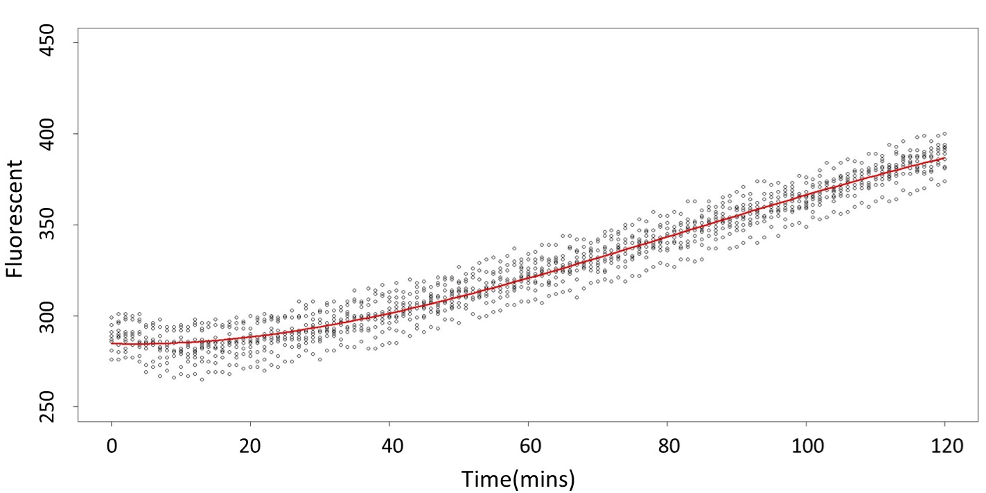
(summary)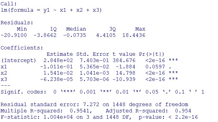
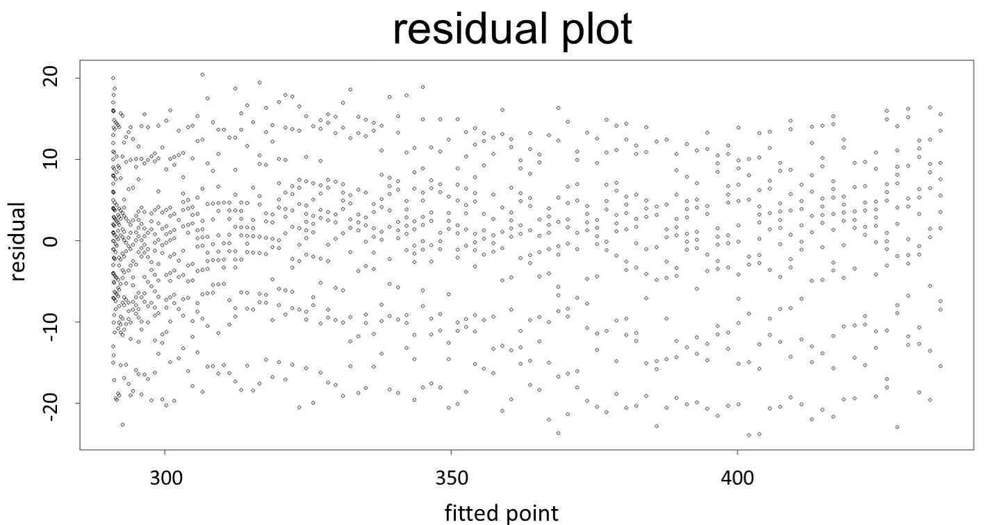
(residual plot) [2]
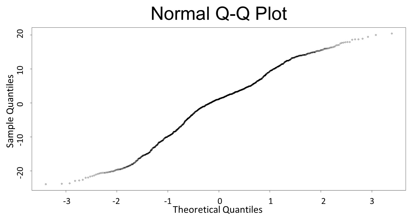
(Q-Q plot)

This model conforms the assumption and R-square is equal to 0.9541, so we think the cubic polynomial regression model is suitable.
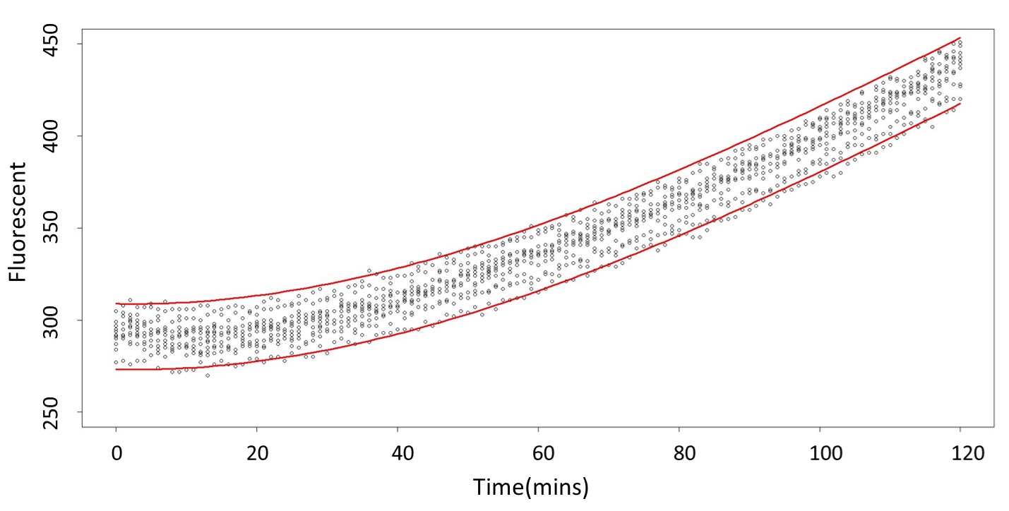
(prediction interval)
Formula: \(\bar{X}\pm t_{\frac{\alpha}{2},n-1}S\sqrt{1+\frac{1}{n}}\)
And the procedure is same in the 5 mM and 120 mM.
(5 mM)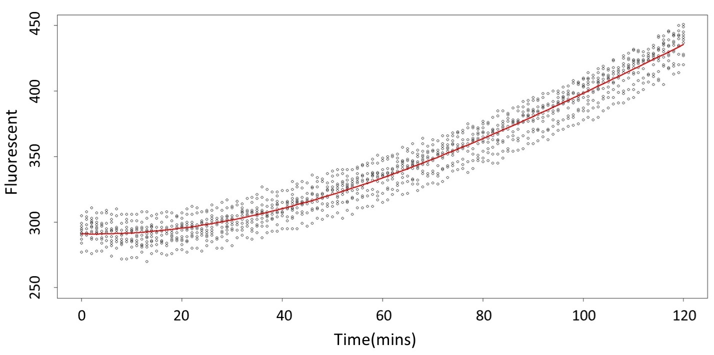
 (120 mM)
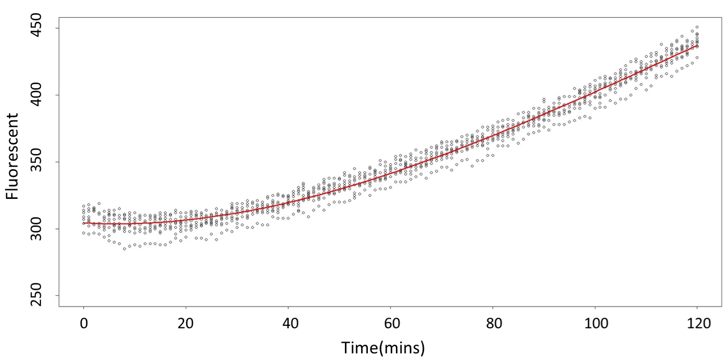
2. According to the paired-difference T test part, it demonstrates that 0.1 mM and 5 mM can be identified as different group due to the statistical significance. In order to precisely distinguish these two groups, choose the time at which the 5 mM and 0.1 mM prediction interval started to diverge to be the recommended prediction time.
Based on the above tables, it showed a significant degree of accuracy when an intersection upon the maximum fluorescence intensity at 0.1 mM and the minimum fluorescence intensity at 5 mM occurs after 101 mins (t> 101 mins). Hence, it can be expected to have higher accuracy of data after 101 mins.
(prediction interval of 0.1 &5 mM)
3. As same as Procedure 2, we choose the time at 120 mM and 0.1 mM prediction interval to diverge to be the recommended prediction
According to the above tables, it showed a significant degree of accuracy when an intersection upon the maximum fluorescence intensity at 5 mM and minimum fluorescence intensity at 120 mM occurs after 88 mins (t> 88 mins). Hence, it can be expected to have higher accuracy of data after 88 mins.
(prediction interval of 0.1 &120 mM)
[1]MONTGOMERY D., et al., Introduction to linear regression analysis, Chapter 2-4 (2012)
[2]Mansfield ER., et al., Diagnostic value of residual and partial residual plots, Journal of The American Statistician (1987)
#0.1 vs 5
#0.1 urine plot
data<-read.csv("C:/Users/Rick/Desktop/NCKUactivity/iGEM/819test/0.1urine.csv",header=T)
x1<-rep(data[,1],12)
x2<-x1^2
x3<-x1^3
y1<-c(data[,2],data[,3],data[,4],data[,5],data[,6],data[,7], data[,8],data[,9],data[,10], data[,11],data[,12],data[,13])
model<-lm(y1~x1+x2+x3)
yhat0.1<-model$fit
plot(x1,y1,ylim=c(250,450),xlab= "time(mins) ",ylab= "Fluorescent", cex.lab=1.5)
#lines(data[,1], yhat0.1[1:121],lwd=3,col=2)
n=121*12
mse<-sum((y1-yhat0.1)^2)/(n-3)  # calculate MS_Res(=σ^2)
X<-cbind(1,x1,x2,x3)
se<-sqrt(mse*(1+X[1,]%*%solve(t(X)%*%X)%*%X[1,]))
up0.1<-model$coefficients[1]+x1*model$coefficients[2]+x2*model$coefficients[3]+x3*model$coefficients[4]+qt(.975,df=n-2)*se
low0.1<-model$coefficients[1]+x1*model$coefficients[2]+x2*model$coefficients[3]+x3*model$coefficients[4]+qt(.025,df=n-2)*se
lines(data[,1], up0.1[1:121], col=2,lwd=3)
lines(data[,1], low0.1[1:121],col=2,lwd=3)
#5 urine plot
data<-read.csv("C:/Users/Rick/Desktop/NCKUactivity/iGEM/819test/5urine.csv",header=T)
x1<-rep(data[,1],12)
x2<-x1^2
x3<-x1^3
y1<-c(data[,2],data[,3],data[,4],data[,5],data[,6],data[,7], data[,8],data[,9],data[,10], data[,11],data[,12],data[,13])
model<-lm(y1~x1+x2+x3)
yhat5<-model$fit
par(new=TRUE)
plot(x1,y1,ylim=c(250,450),xlab= "time(mins) ",ylab= "Fluorescent", cex.lab=1.5)
#lines(data[,1], yhat5[1:121],lwd=3,col=2)
n=121*12
mse<-sum((y1-yhat5)^2)/(n-3)  # calculate MS_Res(=σ^2)
X<-cbind(1,x1,x2,x3)
se<-sqrt(mse*(1+X[1,]%*%solve(t(X)%*%X)%*%X[1,]))
up5<-model$coefficients[1]+x1*model$coefficients[2]+x2*model$coefficients[3]+x3*model$coefficients[4]+qt(.975,df=n-2)*se
low5<-model$coefficients[1]+x1*model$coefficients[2]+x2*model$coefficients[3]+x3*model$coefficients[4] +qt(.025,df=n-2)*se
lines(data[,1], up5[1:121], col=3,lwd=3)
lines(data[,1], low5[1:121], col=3,lwd=3)
title(main="0.1 vs 5mM",cex.main=4)
Name<-c(expression(paste("0.1mM")),expression(paste("5mM")))
legend("topleft", Name, ncol = 1, cex = 1.5, col=c("red","green"),lwd = c(2,2), bg = 'gray90')
#0.1 vs 120
#0.1 urine plot
data<-read.csv("C:/Users/Rick/Desktop/NCKUactivity/iGEM/819test/0.1urine.csv",header=T)
x1<-rep(data[,1],12)
x2<-x1^2
x3<-x1^3
y1<-c(data[,2],data[,3],data[,4],data[,5],data[,6],data[,7], data[,8],data[,9],data[,10], data[,11],data[,12],data[,13])
model<-lm(y1~x1+x2+x3)
yhat0.1<-model$fit
plot(x1,y1,ylim=c(250,450),xlab= "time(mins) ",ylab= "Fluorescent", cex.lab=1.5)
#lines(data[,1], yhat0.1[1:121],lwd=3,col=2)
n=121*12
mse<-sum((y1-yhat0.1)^2)/(n-3)  # calculate MS_Res(=σ^2)
X<-cbind(1,x1,x2,x3)
se<-sqrt(mse*(1+X[1,]%*%solve(t(X)%*%X)%*%X[1,]))
up0.1<-model$coefficients[1]+x1*model$coefficients[2]+x2*model$coefficients[3]+x3*model$coefficients[4]+qt(.975,df=n-2)*se
low0.1<-model$coefficients[1]+x1*model$coefficients[2]+x2*model$coefficients[3]+x3*model$coefficiens[4]+qt(.025,df=n-2)*se
lines(data[,1], up0.1[1:121], col=2,lwd=3)
lines(data[,1], low0.1[1:121],col=2,lwd=3)
#120 urine plot
data<-read.csv("C:/Users/Rick/Desktop/NCKUactivity/iGEM/819test/120urine.csv",header=T)
x1<-rep(data[,1],10)
x2<-x1^2
x3<-x1^3
y1<-c(data[,2],data[,3],data[,4],data[,5],data[,6],data[,9],data[,10],data[,11],data[,12],data[,13])
model<-lm(y1~x1+x2+x3)
yhat120<-model$fit
par(new=TRUE)
plot(x1,y1,ylim=c(250,450),xlab= "time(mins) ",ylab= "Fluorescent", cex.lab=1.5)
#lines(data[,1], yhat120[1:121],lwd=3,col=2)
n=121*10
mse<-sum((y1-yhat120)^2)/(n-3)  # calculate MS_Res(=σ^2)
X<-cbind(1,x1,x2,x3)
se<-sqrt(mse*(1+X[1,]%*%solve(t(X)%*%X)%*%X[1,]))
up120<-model$coefficients[1]+x1*model$coefficients[2]+x2*model$coefficients[3]+x3*model$coefficients[4]+qt(.975,df=n-2)*se
low120<-model$coefficients[1]+x1*model$coefficients[2]+x2*model$coefficients[3]+x3*model$coefficients[4]+qt(.025,df=n-2)*se
lines(data[,1], up120[1:121], col=4,lwd=3)
lines(data[,1], low120[1:121], col=4,lwd=3)
title(main="0.1 vs 120mM",cex.main=4)
Name<-c(expression(paste("0.1mM")),expression(paste("120mM")))
legend("topleft", Name, ncol = 1, cex = 1.5, col=c("red","green"),lwd = c(2,2), bg = 'gray90')