| Line 1: | Line 1: | ||
{{LMU-TUM_Munich|navClass=model}} | {{LMU-TUM_Munich|navClass=model}} | ||
[[File:Muc16_Sticker_Model_001.png |right|500px]] | [[File:Muc16_Sticker_Model_001.png |right|500px]] | ||
| − | |||
= Crosslinking Model = | = Crosslinking Model = | ||
Revision as of 14:10, 3 December 2016
Contents
Crosslinking Model
Since our approach to tissue printing is supposed to work without a supporting scaffold, the cohesiveness of the printed medium is crucial. Biotin binds strongly to Streptavidin as well as Avidin. Thus we are not worried about the individual bonding itself but rather about the interconnectedness of the individual cells and binding .
Nomenclature
Before diving into the details we introduce a few abbreviations to make reading and writing more easy and efficient. Since it is yet to decide weather Streptavidin/Avidin or Biotin will be attached to the cells or to the networking (NP) we refer to the binding sites of cells as CBS and to the ones of NP as NPBS.
Problem definition
In the worst case all CBS we dispense from the printhead would get immediately occupied with otherwise loose NP, which would leave us with lots of individual NP-coated cells. The other extreme case would be that that the cell hardly finds any to bond to. Again resulting in individual cells that are unconnected.
First attempt
So we assumed that the problem is most likely a typical question of polymerization. While the bonds in our case are not covalent we decided it should be safe to assume they were, since they are very strong with a dissociation constant of 10-15 M. So our most promising discoveries after browsing pertinent literature were the Carothers equation as well as the Flory-Stockmayer theory, which is a generalization of the former, which gets closer to what we need, since the Carothers equation assumes that all monomers are bivalent.[1] The Flory-Stockmayer Theory assumes there are 3 different Monomers.
- bivalent units of type A
- multivalent units of type A and
- bivalent units of type B
Further it assumes that B units can only react with A units and vice versa. So by setting the concentration of bivalent A units to 0 we get quite close to the setup we have. However the Flory Stockmayer theory only asses whether gelation occurs or not. Without providing information on how fast or how well it will turn out. [2]
After we found that the results provided are not sufficient to optimize our process we were talking to some Professors in the field of polymer chemistry, biochemistry and biological modelling. Most Answers were discouraging, because to our surprise none of them ever heard of a existing model that would solve (part of) our problem. Ultimately we decided to pursue the advice of Dr. Hasenauer, who suggested to program a simulation of the problem in order to understand it better. First a simple simulation with strong assumptions, later on reducing them step wise to get more and more accurate results.
First simulation setup
So our first approach assumed:
- Every cell has x CBS.
- Every NP has y PBS.
- There are 100 cells and z NP.
- Every pair of CBS and PBS have the same probability to bind. Regardless of spacial distance, obstruction or timing.
- At some point either all or all cell binding sites will have bond.
Results
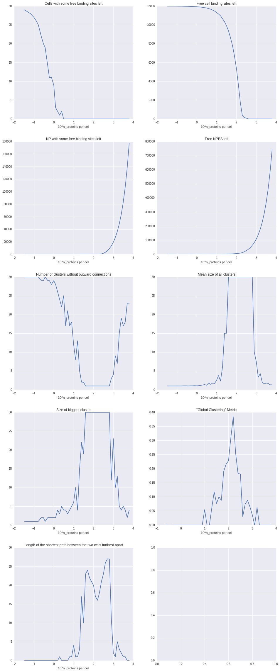
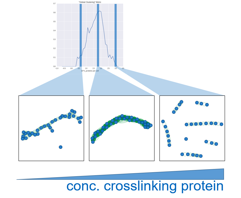
In a first experiment we fixed x to 30, compromising between a way higher number of binding sites, which could “consume” , and a much lower amount of cells that could actually surround it due to spacial limitations. Furthermore we fixed y to 8 to get a first impression and run experiments with logarithmically varying z (number of NP). To analyze the result we analyzed what we call a cell-graph. The cell-graph is obtained by drawing a node for each cell and connecting each node with an edge to the nodes of the respective other cells that this cell is connected to via a NP. On this graph we evaluated a couple of metrics from graph theory, resulting in the plots you can see in the Code section.
Discussion
We were happy to see that most metrics were pointing to roughly the same sweet spot of relative polymer/cell concentration. Soon we discovered however that the solution is a rather trivial one. Since either all CBS or all NPBS are bond before the simulation stops it’s quite obvious that the sweet spot is where the total combined PBS equal the combined CBS. So next we tried to incorporate spatial effects into binding probability.
Second simulation approach
Again we assume:
- Every cell has x CBS.
- Every NP has y PBS.
- There are 100 cells and z NP.
But instead of assuming equal probability for each CBS/PBS pair to bind we assume:
- A one-dimensional space, where all cells as well as NP are placed in equidistant manner.
- For now the position of individual CBS is assumed equal to the respective cell. Likewise for PBS and NP.
- The size of the space is defined by a constant c, where 1 means that the space is of size 1 and 0.01 means the space is of size 100. This constant corresponds to the concentration of active components in a medium. The lower the concentration the higher the distance between two components.
- At every timestep a constant fraction of free PBS tries to bind. (reactivity)
- When a PBS is trying to react, each free CBS gets assigned a certain probability depending on two principles:
- The more near a CBS is to the NPBS, the more likely it is to bind to this one. So the binding probability is defined by a pdf of the zero mean gaussian of the distance with a certain variance that resembles the spacial range of a NP.
- The more cells are bound to a certain NP already, the less likely it is, that it will bind to one that it didn’t bind to yet. Actually since the cells are so big compared to the NP, that a NP can connect to two cells at most. When it's bound to one cell already we consider the event of a second binding to this cell 10 times higher than to any other cell.
- With increasing time, the variance modeling the range of a NP is increasing in order to model, that cells and NP can move freely in the medium and reach more distant partners. We are neglecting, that the cell will move in either direction and just consider the actual position more and more uncertain, so we increase the variance.
- After a defined number of timesteps the experiment is stopped and the result is assessed the same way as described for the first experimantal setup.
Results
Discussion
Code
Here is a walkthrough / tutorial for the simulation code we used.
Don't be scared, just scroll down, there are even some nice pictures. If you want to see more check out our code on github: https://github.com/Mofef/iGEM-PolySim/ (Or if you have problems with viewing this, there is the same content at github in the file "simulation.ipynb")
Shear Stress Model
A not negligible problem in the bio printing field is a reduced cell viability due to shear stress on cells during the process.
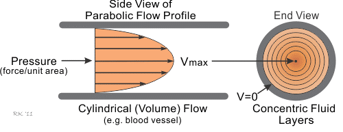
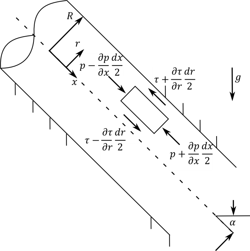
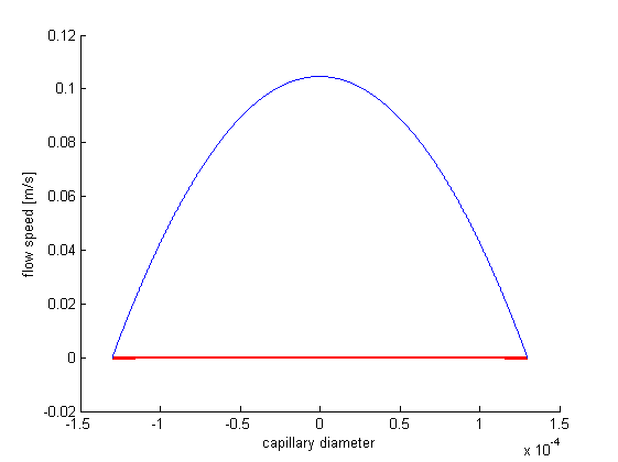
In fluid mechanics, laminar flow is modelled as layers, that can't intersect each other. Due to it's viscosity, layers can transmit forces between them. When observing laminar flow in a straight tube, it can be determined, that due to the wall friction and viscosity of the medium, the volumetric flow speed isn't constant throughout the profile of the tube. It's a parabola-shaped speed distribution with it's maximum in the middle and theoretically no speed at boundary layers. This difference in speed among the layers arises from certain forces in the liquid. Since a layer is a two-dimensional construct, a force can't be attributed to a layer, but to an infinitesimal area, which results in what we are searching for, the shear stress.
As a recent paper[3] concludes, cells maintain near 100% viability rate at up to 5 kPa. In order to verify that we have a sufficient cell viability to print a tissue capable of surviving, we established a mathematical model.
First of all, we had to make sure, that the flow in our system is a laminar one, since it's counterpart, the turbulent flow, isn't as easily calculatable. Since our calculated Reynolds number was significantly smaller than 2000, which is the boundary value between laminar and turbulent flow, we could model the flow as a laminar one.
Our model was derived from the differential relationships in a fluid.
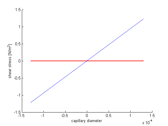
With the constraint that all forces in direction of the pipe are zero, for there are no accelerations by definition, we can formulate a differential equation. It's solution delivers the formula for the laminar flow speed distribution over the pipe's diameter. It's derivative can be inserted in newton's formula that can be applied in incompressible isotropic cases and delivers the shear stress as a function of the pipe's diameter. When this is applied to the Hagen–Poiseuille equation, we get a shear stress diagram dependent on the volumetric flow speed. The following Matlab program was used to calculate and display our results.
r=-0.00013:0.0000001:0.00013; %plot vector radius
v=10/(3.6*10^9); %volume flow
p=(8*1.52*10^-3*v*0.62)/(pi*0.00013^4); %resulting pressure
hold on;
viscircles([0,0],max(r)); %circle for capillary visualization
plot(r,-1/(4*1.52*10^-3)*(p/0.62)*(r.^2-0.00013^2)); %plot of volume flow profile
xlabel('capillary diameter')
ylabel('flow speed [m/s]')
figure;
hold on;
viscircles([0,0],max(r));%circle for capillary visualization
plot(r,-1/4*(p/0.62)*(0.00013^2-r)); %plot of shear stress profile
xlabel('capillary diameter')
ylabel('shear stress [N/m^2]')
MaxShearStress=max(1/4*(p/0.62)*(0.00013^2-r))%maximum of the resulting shear stress vector
MaxShearStress =

    1.2236
As you can see in the figure, shear stress doesn’t exceed a boundary of 1.3 N/m^2 (Pa). According to the aforementioned paper, the cell viability should be near 100%.
References
- ↑ Wikipedia: Carothers equation
- ↑ Wikipedia: Flory-Stockmayer Theory
- ↑ Blaeser, Andreas, et al. "Controlling shear stress in 3D bioprinting is a key factor to balance printing resolution and stem cell integrity." Advanced healthcare materials 5.3 (2016): 326-333.


