Team:HZAU-China/Model


The density distributions of bacteria in culture medium depends on two factors: motility and multiply of bacteria. For convenience, we will discuss these two factors separately.
motility dynamic model
In this project, we are trying to control the motility of bacteria by control the light matrix to make a colony with a specific shape. That the light matrix can affect the motility of bacteria is by influencing the expression of a protein related with motility and this protein is chez in this project. There are two forms of bacterial motility: tumbling and swimming. By tumbling, bacteria can change its swimming direction but not position. But by swimming, bacteria will forward to change its position. In fact, the rate of tumbling and swimming is different from bacteria to bacteria. At the micro level, the angle of tumbling is random, so we have no idea the movement direction of bacteria in any time. But in the view of macroscopic, the probability of all directions are equal. This property is similar to the diffusion of chemical. So, the swimming of bacteria can be seen as the diffusion of bacteria and the rate of diffusion is related to expression of chez.
Due to the multiply of bacteria makes little difference to the diffusion, so we don’t consider the multiply of bacteria provisionally.
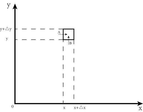
(Figure1. Simple graph about diffusion of bacteria.)
In Figure 1, the simple square represent the area of bacterial in coordinate \((x,y)\) approximatively. The number of bacteria in this area is \(S(x,y,t)\) at time t. So, we have:
\(S(x,y,t)=\rho(x,y,t)*\Delta x\Delta y\) \((1)\)
In equation \((1)\), \(\rho(x,y,t)\) represent density of bacteria in that area. \(\Delta x\) and \(\Delta y\) are the smallest increment in the \(x\) and \(y\) axis respectively. After taken the derivative of equation (1), we have:
\(\frac {\partial S(x,y,t)}{\partial t}=\frac {\partial\rho(x,y,t)*\Delta x\Delta y}{\partial t}\) \((2)\)
The left part of equation \((2)\) represent the change rate of \(S(x,y,t)\). Under the premise of ignore the multiply of bacteria, the change rate depends on the rate of diffusion of bacteria. As shown in Figure 1, bacteria can move along the \(x\) axis and \(y\) axis. Limit that along the \(x\) and \(y\) axis is the positive. So:
\(\frac {\partial\rho (x,y,t)\Delta x\Delta y}{\partial t}=\phi_x(x,y,t)\Delta y- \phi_x(x+\Delta x,y,t)\Delta y+\phi_y(x,y,t)\Delta x-\phi_y(x,y+\Delta y,t)\Delta x\) \((3)\)
In equation \((3)\), \(\phi_x\) and \(\phi_y\) represent the diffusion of bacteria in \(x\) and \(y\) axis respectively. Dividing \(\Delta x*\Delta y\) on both sides of equation \((3)\), and we can get:
\(\frac {\partial\rho(x,y,t)}{\partial t}=\frac {\phi_x(x,y,t)-\phi_x(x+\Delta x,y,t)}{\Delta x}+\frac {\phi_y(x,y,t)-\phi_y(x,y+\Delta y,t)}{\Delta y}\) \((4)\)
In fact, equation \((4)\) is not a strict equation because \(\Delta x\) and \(\Delta y\) are not minimum value. But if let \(\Delta x\) and \(\Delta y\) take a limit to 0, equation \((4)\) will be an equation. So we have:
\(\frac {\partial\rho(x,y,t)}{\partial t}=\lim_{\Delta x\rightarrow 0}\frac {\phi_x(x,y,t)-\phi_x(x+\Delta x,y,t)}{\Delta x}+\lim_{\Delta x\rightarrow 0}\frac {\phi_y(x,y,t)-\phi_y(x,y+\Delta y,t)}{\Delta y}\) \((5)\)
This equation is equivalent to:
\(\frac{\partial \rho}{\partial t}=-(\frac{\partial\phi_x}{\partial x}+\frac{\partial\phi_y}{\partial y})\) \((6)\)
Here, we omit the coordinates. In this equation, \(\phi_x\) and \(\phi_y\) is difficult to be known by us. In fact, the rate of diffusion in \(x\) and \(y\) axis is same. From the assumption of Fourier Heat Equation:
1. If the temperature is constant within an area, there is no flow of heart.
2. If the temperature difference exists in adjacent area, heart will flow from areas high to low.
3. For the same kind of material, the bigger the temperature difference of two adjacent area, the faster flow between them.
Similarly, the three characters are suitable in bacteria colony:
1. If the density of bacteria is constant in an area, the move of bacteria will not lead to the change of density.
2. If the density difference exists in adjacent area, bacteria will swim from high density to low density area on the macro.
3. The bigger the density of two adjacent area, the faster diffusion between them.
So, the rate of diffusion is related with the difference of density:
\(\phi_x = -k\frac{\partial\rho}{\partial x}\) \((7)\)
\(\phi_y = -k\frac{\partial\rho}{\partial y}\) \((8)\)
Combining equation\((7)\) and equation\((8)\) with equation\((6)\), we can get:
\(\frac{\partial\rho}{\partial t} = k(\frac{\partial^2\rho}{\partial x^2}+\frac{\partial^2\rho}{\partial y^2})\) \((9)\)
Multiply model
There is a famous model about the growth states of bacteria under the condition of limited space and nutrients called logistic growth model:
\(\frac{d\rho}{dt} = \gamma\rho(1-\frac{\rho}{\rho_s})\) \((10)\)
In equation \((10)\), \(\rho\) represent the density of bacteria, and \(\gamma\) is growth rate constant, and \(\rho_s\) is saturated density.
Multiply and motility dynamic model of bacterial
Combining equation \((9)\) with equation \((10)\), we have:
\(\frac{\partial\rho}{\partial t}=k(\frac{\partial^2\rho}{\partial x^2}+\frac{\partial^2\rho}{\partial y^2})+\gamma\rho(1-\frac{\rho}{\rho_s})\) \((11)\)
Reference Chenli liu et al, we have several parameter values,
$$k=200~1000\mu m^2/s$$ $$\gamma = 3.89e-4s^{-1}$$ $$\rho_s = 1500cell/\mu m^2$$
We will use finite element method to solve this PDE. Defining initial conditions are,
$$\rho=matrix.zeros(200,200)$$ $$\rho[100,100]=100$$
\(matrix.zeros(200, 200)\) means a zero matrix with \(200*200\), and the value of the index \([100, 100]\) of this matrix is \(100\). And the boundary conditions are,
$$\rho[0:,]=0$$ $$\rho[100:,0]=0$$ $$\rho[0,0:]=0$$ $$\rho[0,100:]=0$$
Writhing solve program with python and numpy to solve equation \((11)\), and the result was showed by mayavi, then we can get a video that can be seen in Movie1.
(Movie1)
Multiply and motility dynamic model under the condition of restricted area
In Movie1, we can see that colony will be a roundness eventually. If we add a restrictive condition about the area that bacteria can move, then what the colony will become? The way to add area limit is using light to control the motility of bacterias. So we will give green light in a specific area and the remainder will be given red light. And bacterias can move only in this green light area. In equation (11), Bacterial motility is mirrored by parameter k. So the model will be the following equations.
\(\frac{\partial\rho}{\partial t}=k(\frac{\partial^2\rho}{\partial x^2}+\frac{\partial^2\rho}{\partial y^2})+\gamma\rho(1-\frac{\rho}{\rho_s})\) \((11)\)
\(k=f(x,y)\) \((12)\)
\(k\) in equation \((11)\) means the diffusion rate of colony. \(f(x,y)\) is area limit function, and it’s an image matrix. In this project, we choose Pikachu who is a famous role in a hot AR game Pokimon Go. See this picture in Figure2.

(Figure2)
The black part in Figure2 means that the parameter \(k\) is normal value. That is \(k=k_normal=200~1000\mu m^2/s\). And the white part in Figure2 means that the parameter \(k\) is a small value which will be set to \(0\). But \(k\) is a matrix in equation \((11)\), and it can be solved out using Figure2.
$$k = img*k_normal/255$$
Under the aforementioned initial conditions and boundary conditions, using python program to solve these equations.
(Movie2)
From Movie2 we can see that a specific pattern is basically formed. But such a pattern formation is just equivalent to using mould. In this project, the pattern formation will be adjusted by computer in real time.
Multiply and motility dynamic model with dynamic regulation
Area limit is static regulation, but dynamic regulation is more suitable in our expectation. In dynamic regulation, we will compare the shape of colony with target picture in real time, and the result of comparing will be converted to light matrix to be irradiate on colony. So, the dynamic model will like the following context.
\(\frac{\partial\rho}{\partial t}=k(\frac{\partial^2\rho}{\partial x^2}+\frac{\partial^2\rho}{\partial y^2})+\gamma\rho(1-\frac{\rho}{\rho_s})\) \((11)\)
\(k=f(t,\rho,img)\) \((13)\)
Unlike equation\((12)\), there are two additional parameters in equation\((13)\). The two additional parameters are time \(t\) and density \(\rho\) respectively. That means parameter \(k\) will be change in the process of adjustment. And equation\((13)\) can be interpreted as,
\(\rho_1=\rho*\frac{255}{max(\rho)}\) \((14)\)
\(\rho_2=threshold(\rho_1,THRES_BINARY_INV)\) \((15)\)